English (pdf)
 Article in xml format
 Article references
 Send this article by e-mail
 Cited by SciELO
  Cited by Google
  Similars in
SciELO
Similars in
SciELO  Similars in Google
 Permalink
1. Introduction
Tremendous agricultural potential in Colombia has gone untapped for decades due to a myriad of factors, including: i) civil strife and the criminal drug trade; ii) uncertainty regarding property rights; iii) inadequate infrastructure; iv) lack of innovation and technological development; v) lack of access to funding, vi) lack of investment; and vii) misallocation of resources within the sector (COMPITE, 2008; Clavijo, Vera & Fandiño, 2013; Junguito, Perfetti, & Becerra, 2014; and Reina, Zuluaga, Bermúdez & Oviedo, 2011). Government policies have allocated economic and development efforts to urban and industrial areas (e.g. financial, mining and utilities) rather than rural agricultural areas, where insurgent forces have often taken refuge (Junguito et al., 2014).1 It was generally the case that when agricultural policies were implemented, they were done so with short-term goals in mind (SAC, 2014). With recent advances toward peace between the Colombian government and insurgents as well as less incidences of drug trafficking in the country, Colombia is poised for renewed public and private investment in agriculture and rural communities.2This agreement may well improve the environment of agricultural investment, and the return of combatants and others to rural activities means not only a greater labor supply, but also that agriculture must play a key role in future national development. The results presented in this paper have the potential to inform better policies toward rural and agricultural development in Colombia in the post-conflict era.
The value of Colombia’s agricultural production grew by only 10% during the agricultural commodity price booms of 2006-2011, relative to its average growth from 2000-2005. In contrast, the value of global agricultural production expanded by 25%, and much greater growth occurred in other Latin American countries: 26.1% in Chile, 28.6% in Argentina, 43.6% in Brazil and 45.6% in Peru (FAO, 2015). We analyze the relatively weak performance of Colombia’s agriculture and evaluates whether it was due to a low productivity growth rather than a lack of input accumulation. Our general hypothesis is that deep structural problems, suggested by low productivity growth rates, prevented Colombia’s agriculture from exhibiting the higher growth of the commodity prices booms.
Previous investigations suggest that over recent decades Colombia’s agriculture has exhibited stagnant growth of between 1.5% and 2% per year (World Bank, 2016), mainly due to the structural problems mentioned above. Likewise, Colombia’s agriculture has been subject to many distortions due to agricultural policy design and administration which limited the country’s competitiveness (Anderson and Valdés, 2008). Moreover, public expenditure on Colombia’s agriculture has represented just 0.2-0.4% of overall GDP since the late 1990s, while this figure has reached 1% in other emerging markets and 4% in developed countries (Junguito et al., 2014). These deep structural problems leading to slower agricultural sector growth have varied over time due to political and economic circumstances leading to variations in both productivity growth and input accumulation.
In contrast, prices received by Colombian farmers increased by 30% in 2008 and 57% in 2011 relative to average prices from 2000-2005 according to the Producer Price Index (PPI) calculated by the Departamento Administrativo Nacional de Estadística (DANE, 2015). Accordingly, Colombia’s farmers surely experienced the effects of high global commodity prices seen in 2008 and 2011. Then, farmers were exposed to incentives to increase both their productivity and input use. However, the aforementioned structural problems seem to have prevented Colombia from reaching a higher standard of agricultural performance.
Colombia’s agricultural productivity has rarely been analyzed in the economics literature, and the techniques used to measure its agricultural productivity have been inconsistent (Atkinson, 1970; Avila et al., 2010; Ludena, 2010; Pfeiffer, 2003; USDA, 2015). Most of these studies have relied on accounting methods, employing untested assumptions rather than econometric estimation, and substituting data from neighboring countries for missing Colombian data. Likewise, these studies did not reach a consensus and are essentially incomparable because they address different time periods, employ different data sources, and/or employ contradictory underlying assumptions.
One contribution of this paper is that it econometrically measures Colombia’s agricultural productivity growth, both aggregated and disaggregated for crop and livestock production during the period 1975-2013.3 We employ three commonly used econometric specifications to analyze the robustness of results to alternative specifications and their associated underlying assumptions about technology, etc. One of these is a Translog Cost function model that allows for the investigation of bias in technical change and scale effects, as well as providing confidence intervals for the productivity estimates (Antle and Capalbo 1988). The other two specifications are the Cobb-Douglass and the CES production technologies. A second contribution is that this paper assembles a current and complete Colombia dataset that does not feature data substitution from neighboring countries. Thus, this study assesses how Colombia’s agricultural productivity growth has changed over time relative to varying policy regimes and economic circumstances. To this aim, we conduct a historical analysis of Colombia’s agriculture from 1975-2013 that models six key structurally different time periods, during which economic conditions and policy regimes strongly influenced agricultural productivity growth (see Table 1).
This paper proceeds as follows. Section 2 describes the overall context for Colombia’s agriculture from 1975-2013. Section 3 presents a review of the relevant literature on Colombia and the most common methodologies used to measure agricultural productivity. Section 4 explains the methodology used in this study. Section 5 describes the data used. Section 6 analyzes the various agricultural productivity growth estimates for Colombia obtained by the current study. Section 7 provides our concluding remarks.
2. Colombia’s agriculture from 1975-2013
Agriculture is one of the most important economic activities of Colombia. About 40% of Colombia’s land is used for agricultural purposes. Agricultural GDP has averaged 6-8% of Colombia’s total GDP and agricultural exports account for 18% of total national exports in recent decades (DANE, 2015). Moreover, agriculture employs 20% of the national labor force and 66% of the rural labor force (COMPITE, 2008; SAC, 2011; DANE, 2015). Colombia increased the value of its production by 50% in the last two decades, ensured its self-sufficiency in agricultural products, and consolidated a diverse portfolio of products (e.g., beef, milk, chicken, sugar cane, coffee and flowers) for domestic consumption and exportation (FAO, 2015).
However, Colombia’s agriculture has been seriously affected by a significant lack of investment in recent decades (Junguito et al., 2014). Likewise, the transformation of Colombia’s economy into an oil-dependent economy after the discovery of Caño Limon in 1983 and Cusiana-Cupiagua in 1991 (two great oil deposits) damaged the competitiveness of tradable sectors, among them agriculture. Moreover, Colombia’s agriculture has tackled all the aforementioned structural problems, which undoubtedly has limited performance. Consequently, Colombia’s agricultural GDP has exhibited a significant slowdown, from an annual average growth of 4.5% in the 1970s, 2.7% in the 1980s, 1.5% in the 1990s, and 1.9% in the 2000s (World Bank, 2016).
Looking forward, agriculture in Colombia is a sector with promising prospects in the coming decades. Along with Brazil, the Congo, Angola, Sudan, and Bolivia, Colombia is one of the few countries with the opportunity to expand its agricultural frontier (FAO, 2013). The Orinoco region, similar to the Cerrado in Brazil, would allow Colombia to expand its farmland by 80% (between 3-5 million hectares) if Colombia improves its infrastructure and prioritizes the development of new agricultural technologies in the region (Clavijo & Jimenez, 2011c). Accordingly, Colombia has the potential to become a global exporter of agricultural products, given that: i) the United Nations predicts the world population will grow by 30% to 9,100 million people (2% per year) by 2050 (UN, 2015); ii) the Food and Agriculture Organization (FAO) estimates that global food production must increase by 70% (5% per year) to feed the growing population (FAO, 2009); iii) Colombia’s agricultural GDP per capita will grow on average by 2-4% in the coming decades; and iv) Colombia’s agricultural GDP is projected to grow 4-5% annually and its population is projected to grow by only 1-1.5% annually, according to official predictions (DANE, 2015; MADR, 2014).
3. Measurement of Agricultural Productivity
3.1 Theoretical Framework
Agricultural productivity has been widely measured worldwide, beginning with the pioneering work of Solow (1957) and Griliches (1963 a-b, 1964). Productivity has been recognized as an essential source of growth that encompasses the output gains attributable to technical change (Pfeiffer, 2003). Development economists have also stated that agricultural productivity is particularly critical to developing countries’ improved economic growth and social conditions (Johnson and Mellor, 1961). In addition, studies have also shown that agricultural productivity is a key factor explaining the dynamics of worldwide trade, by determining changes in the comparative advantages among countries (Ball et al., 2010). Accordingly, agricultural productivity has been the focus of a significant number of studies (Ball, 1985; Fernandez-Cornejo and Shumway, 1997; Avila et al., 2010; Evenson & Fuglie, 2010; Fuglie & Rada, 2013 to name a few).
Three different methodology types are often used to measure agricultural productivity. The first is growth accounting. This technique measures agricultural productivity by following a simple accounting exercise (Solow, 1957): aggregate output growth is estimated as the growth of the value of all outputs; aggregate input growth is measured as a cost share weighted average of the growth in inputs used in production of the various outputs; and productivity growth is identified as the residual difference between these two measures.4
The simple exercise makes the growth accounting technique very attractive. However, the technique relies on very strong assumptions: i) competitive markets for both outputs and inputs; ii) constant returns to scale; iii) technical change is Hicks neutral; iv) input-output separability; and v) a Cobb-Douglas production function (Antle and Capalbo, 1988; Diewert, 1992).5 6 7 Many studies have used these techniques and the USDA relies on this methodology for measuring International Agricultural Total Factor Productivity (TFP) Growth (Evenson and Fuglie, 2010; Fuglie, 2010; Fuglie and Rada, 2013; Rada, 2013).
Superlative index methods have been used to relax these assumptions. The most commonly used are the Tornqvist- Theil Index (Ball, 1985; Evenson et al., 1999; Fan and Zhang, 2002; Garcia et al., 2012; Thirtle et al., 2008) and the Fisher Index (Cahill and Rich, 2012; Zhao et al., 2012). These procedures measure the agricultural productivity without estimating a functional structure for the production function for long periods of time. However, these methods are data demanding, and their economic interpretation is not always intuitive (Saikia, 2009). In addition, productivity estimates largely depend on the index number formula (Diewert and Nakamura, 2002).
Another methodology is the frontier technique (Farrell, 1957). These techniques rely on the fact that economic activities may not always be located in their best practice frontiers (i.e. on the Production Possibility Frontier, or PPF) (Coelli, Rao and Battesse, 1998).8 Accordingly, agricultural productivity corresponds to the estimation and posterior product of two components: technical change, which captures shifts in the production possibility frontier, and efficiency change, which considers movements exhibited by a firm or economic activity within its production possibility set toward a position closer to that frontier (Sena, 2013). Hence, agricultural productivity measurement largely depends on a robust estimation of the production possibility frontier and the corresponding estimation of these two components using the frontier as an efficiency benchmark.
Two frontier types are primarily utilized for the measurement of agricultural productivity: i) parametric methods, such as Data Envelopment Analysis (DEA) and Stochastic Frontier Analysis (SFA) (Coelli, Rao and Battesse, 1998), and ii) non-parametric methods, such as the Malmquist Index (Caves et al., 1982). These techniques are very attractive when data is a constraint, because they do not require any price data (Coelli and Rao, 2005; Sena 2003). However, they are susceptible to data quality issues and unusual shadow prices (Coelli and Rao, 2005; Thirtle et al., 2003; Tong et al. 2012).
Econometric techniques are another common approach used to measure agricultural productivity (Berndt and Christensen, 1973). These techniques assume that productivity can be directly measured when assuming a functional approximation of the true production relationship (so-called primal techniques) or indirectly measured from its Dual Cost function (so-called dual techniques), which requires the functional approximation of the cost or profit function. The main advantages are that econometric models allow: i) relaxing certain assumptions required by accounting approaches, such as Hicks neutral technical change or constant returns to scale; ii) estimating rather than assuming certain parameters related to technical changes, such as the elasticity of factor substitution; and iii) estimating confidence intervals around the estimates and testing hypotheses on the estimated parameters. However, these primal econometric models require a production function with input- output separability, as do growth accounting approaches. Primal econometric models also require a large enough data set to ensure sufficient degrees of freedom, address multi-collinearity problems and estimate a large number of parameters with good precision. Nevertheless, these techniques estimate productivity growth with fewer constraining assumptions than required by other approaches. Econometric models have been successfully used by several studies devoted to analyzing agricultural productivity. For example: Cungu and Swinnen, 2003; Fan, 1991; Sun et al., 2009.
3.2 Agricultural Productivity in Colombia
Colombia’s agricultural productivity has been the focus of just a few studies at the national level (Atkinson, 1970; Avila et al., 2010; Ludena, 2010; Pfeiffer, 2003; USDA, 2015). It has usually been analyzed in the context of multi-national studies (Bravo-Ortega and Lederman, 2004; Coelli and Rao, 2005; Fuglie, 2015; Fulginiti and Perrin, 1998; Trueblood and Coggins, 2003). Relatively little is known about its dynamics over the last several decades.
Atkinson (1970) is the pioneering scholar of Colombia’s agricultural productivity. Using partial productivity indices for the period of 1950-1967, he found that Colombia’s agricultural productivity was uneven across crops and largely dependent on farms’ ability to mechanize their production practices. Also, large farms usually exhibited higher agricultural productivity than small farms, because large farms could afford to pay for better seeds, pesticides and fertilizers.
In more recent studies, growth accounting techniques have been the most common methodology used to measure Colombia’s agricultural productivity. For instance, the USDA (2015) used the technique for 173 countries from 1961-2012. The study estimated that Colombia’s agricultural productivity grew 1.4% on average per year during this period. Avila et al. (2010) used a Tornqvist-Theil Index to examine Colombia’s agricultural productivity between 1961 and 2001 and estimated that it grew an annual average of 0.7%. However, these studies reached different conclusions and none used budget data from Colombian farmers.9
Ludena (2010) used a frontier approach and found that Colombia’s agricultural productivity grew an average of 2.4% during the 1980s, 2.5% during the 1990s, and 0.2% from 2000-2007. Likewise, Pfeiffer (2003) estimated that Colombia’s agricultural productivity grew on average between 0.6-1.9% during the period 1972-2000.10
Clearly, these studies obtained varying results from various techniques that provided non-robust estimates for Colombia’s agricultural productivity. As the time frames changed, so did productivity and agricultural performance estimates. These studies indicate that Colombia’s agricultural productivity grew slowly and unevenly over the last several decades. We suspect that this is probably because most studies implicitly assume that changes in economic conditions and policy regimes did not impact Colombia’s agricultural productivity. This paper considers this to be a crucial assumption that accounts for these differences. Therefore, we incorporate important changes in the political economy over time into our analyses of Colombia’s agricultural productivity.
4. Methodology to Measure Agricultural Productivity in Colombia
In order to measure Colombia’s agricultural productivity, Colombia’s agricultural output is assumed to mainly depend on four inputs (capital, labor, fertilizer and animal feed), following the USDA (2015) and given the data availability for the period analyzed in this study (1975-2013). Three functional approximations are estimated for the production technology in an effort to examine the robustness of the results: Cobb-Douglas production function, CES production function and Translog Cost function.
4.1 Cobb-Douglas Production Function
The choice of functional form is a primary issue in the econometric estimation of productivity growth and technical change. The Cobb-Douglas functional form is one of the simplest choices available and has been widely used in applied economics research. The Cobb-Douglas is supported by the same theoretical underpinnings as the growth accounting technique. Rather than use observed farmers’ budget data to estimate all parameters, this approach estimates them econometrically by controlling for other factors and substitution possibilities implied by the data. Assuming that agricultural productivity grows on average at a constant rate g, so A t = A 0 e gt , the Cobb-Douglas representation of aggregate production is:

where Q t is total agricultural output in period t, A 0 is agricultural productivity in the initial period, e is the exponential function, K t is the stock of capital in agriculture in period t, L t is labor hired by agriculture in period t, Ft is fertilizer used by agriculture in period t, S t is animal feed employed by agriculture in period t and u t is the error in measuring output in period t.
Colombia’s agricultural productivity growth over time is measured as the sum of the average growth g and the residuals of the econometric estimation u t , (which have a mean of zero).11 Crop and livestock productivity growth are also separately estimated in this paper following a similar approach. One of the advantages of a specification such as the Cobb-Douglas function is that it can be estimated using Ordinary Least Squares (OLS) after transforming to the linear version of equation (1) with variables expressed in natural logarithms. Serial autocorrelation across the time dimensional residuals was tested using the Durbin-Watson statistic. When this problem was detected, one-period lagged output was added to the regression as a concomitant variable to incorporate inertia into the aggregate cropping patterns, which likely led to the serially-correlated error.
The Cobb-Douglas parameters α, ß, γ and θ can only be interpreted as input cost shares when the following conditions are satisfied: i) perfect competition; ii) firms maximize their profits; iii) perfect information; and iv) constant returns to scale in period t. Constant returns to scale requires the restriction that α + ß + γ + θ = 1 and that all parameters are non-negative. Otherwise, these parameters represent only the marginal effect of each input on agricultural output. In addition, the Cobb-Douglas function is only capable of representing Hicks-neutral technical change.
The rigid structure and underlying assumptions of the Cobb-Douglas specification may not be supported by the Colombian data. Two alternative econometric approaches were also examined, each of which relaxes some of the assumptions discussed above to varying degrees. The Constant Elasticity of Substitution (CES) production function allows the estimation of a constant elasticity of substitution different from one. The CES also allows for the measurement of biased technical change. Dual approaches that specify a cost function allow for further relaxation of the Cobb-Douglas and growth-accounting assumptions. Dual approaches with higher order polynomial forms are the key aspect of this increased flexibility. In this regard, it is not the dual that is important, but the order of the functional form must be polynomial. However, the dual approach facilitates the use of these functional forms because in many of the more interesting cases, such as the translog functional form, it is not self-dual. This implies that it is not possible to solve the profit maximization problem analytically to obtain a closed form system for the direct estimation of the production function (Antle and Capalbo 1988). The dual approach allows the recovery of potentially unknown but well-behaved production technology information by estimating the input demand and output supply functions derived from the Dual Cost function (Christensen and Greene, 1976). Also, this approach enables the measurement of both biased technical change and the potential impact of aggregate scale effects on productivity growth.
4.2 CES Production Function
The CES production functional form was initially designed to analyze the production of economic activity using only two inputs (Arrow et al., 1961). Sato (1967) generalized this production function for n inputs, explaining that it can be estimated assuming two-input nests. In recent decades, debate has focused on how to determine this nested pair of inputs.
This paper followed the approach developed by Klump et al. (2007) and Leon-Ledesma et al. (2011) to measure Colombia’s agricultural productivity assuming a CES production function. We rely on the following normalized structure of a nested CES production function with four inputs and technical change. The primary inputs (i.e. capital and labor) are allocated to the first nest and the intermediate inputs (i.e. fertilizer and animal feed) to the second nest. Also, to circumvent problems related to the Diamond McFadden Impossibility Theorem (Diamond et al., 1978), the efficiency growth exhibited by each input E it is restricted to a constant rate γ i (Klump et al., 2011).
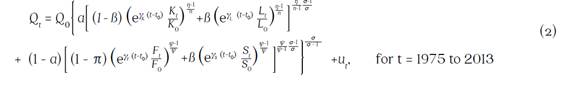
where the elasticity of substitution between capital and labor (i.e. first nest inputs) is η, between fertilizer and feed (i.e. second nest inputs) is ψ, and between nests is σ. Also, α is the distribution parameter between nests, β within the first nest, π within the second, and u t is the error in measuring this CES production function.
The measurement of Colombia’s agricultural productivity involves a typical profit maximization problem to determine the input demands. Each equation derived from this optimization is normalized and linearized. The profit optimization was solved by assuming that Colombia’s agriculture faces a demand function  , its income is Qt = (1+µ)(RtKt +WtLt +fPtFt +sPtSt ) and it exhibits a rent factor
  , where real returns to capital are denoted by Rt, wage paid for labor by Wt, fertilizer price by fPt, and animal feed price by sPt .12 This system of equations was estimated using Iterative Feasible Generalized Non-Linear Least Squares (IFGNLS), as recommended by Kreuser et al. (2015). This technique prevents the estimation of inconsistent parameters and an elasticity of substitution biased towards unity, as is often exhibited when this system of equations is estimated as a Seemingly Unrelated Regression model (SUR) (Luoma and Luoto, 2011).
This model estimated the parameters for technical change γi and input elasticities of substitution (σ,η, and ψ) simultaneously and under two scenarios: i) Hicks-Neutral technical change (γk = γL = γf = γs) and ii) biased technical change (γk ≠ γl ≠ γf ≠ γs). Colombia’s agricultural productivity growth was also measured over time as the actual output growth in period t unexplained by the input growth in period t.
For the measurement of crop and livestock productivity, a similar nested CES production function was used. Crop production was modeled to depend on capital, labor and fertilizer, and livestock production was modeled to depend on capital, labor and animal feed. Accordingly, a nested CES production function with only one nest and an extra input was defined for each case. Also, two possible forms for their respective, nested CES production functions were examined: i) when primary inputs are in the nest or ii) when capital-related inputs are in the nest.13
4.3 TransLog Cost Model
This approach is simpler than using primal methods when price data is available and (as discussed earlier) functional forms of the production function lack a closed form solution to the profit maximization or cost minimization problems. Dual functions, such as a cost or profit function, are valid alternatives to represent the multi-product function and to define the technical change (Antle and Capalbo, 1988).
The effects of technical change can be quantified through a reduction in cost or an increase in profits, given an output level and a set of input prices.
The following translog functional form was specified for the aggregate cost function for Colombia’s agriculture:
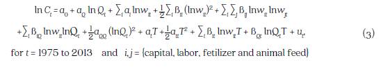
where Ct are the production costs of Colombia’s agriculture in period t, wit is the price of input i in period t, Qt is output in time t, T is a time trend variable that captures technological change and ut is the error in measuring the logarithm of the total cost.
This functional form is a second-order approximation of an arbitrary, twice-continuously differentiable cost function. It exhibits three main strengths: i) flexibility of functional form; ii) does not restrict input substitution possibilities, and iii) scale economies can vary based on output levels (Kant and Nautiyal, 1997; Varian, 1978). The form has been used successfully by other studies in which the production generating dynamic structure was unknown (Binswanger, 1974b; Christensen and Greene, 1976; Clark and Youngblood, 1992; Kant and Nautiyal, 1997; Sun et al., 2009).
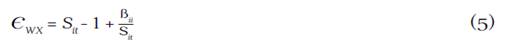
Estimation involves each input i cost share equation, which can be derived by applying Shepard’s Lemma to equation (3).14 Christensen and Greene (1976) explained these equations add additional degrees of freedom to the estimation and do not constrain the coefficients, because it constitutes a multivariate system of equations of i+1 equations where across-equation parameter restrictions create more rapid growth in system degrees of freedom than in parameters as equations that are added to the system. The derived cost share equations take the following form, where Sit is the cost share in period t for input i and εit is the error in measurement of cost share i in period t:
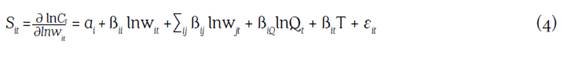
The measurement of Colombia’s agricultural productivity proceeds by estimating this system of equations as a seemingly unrelated regressions (SUR) because a common approximation error is passed to each cost share equation though their residuals (Christensen and Greene, 1976) and the specification of a second order polynomial when the true cost function may be of even higher order. The estimation of the system involves n-1 of the cost share equations due to the adding up restriction of cost shares and associated singularity of the system error variance-covariance matrix.15 Estimated parameters are invariant to which equation is omitted so long as the estimation involves maximum likelihood and the parameters of the omitted equation can be retrieved via the homogeneity and adding up restrictions imposed on the model for regularity purposes. Iterative Feasible Generalized Non-Linear Least Squares (IFGNLS) was used to estimate this system of equations because this estimator is equivalent to a Maximum Likelihood estimator (Greene, 2012).
The following restrictions were imposed to ensure that the corresponding production function is well behaved (Capalbo, 1988; Kant and Nautiyal, 1997): i) coefficients are the same in the cost function and cost share equations; ii) certain coefficients are symmetric among equations; iii) ∑i ai = 1; ∑i ßiQ = 0; and iv) ∑i ßij = ∑j ßji = ∑i ∑j ßij = ∑i ßit = 0 to ensure that this cost function is homogeneous of degree 1 in input prices. Also, curvature restrictions were imposed at the point of the approximation of this cost function (Diewert and Wales, 1987; Ryan and Wales, 2000) and price elasticities for all inputs were computed from estimated parameters using the following expression:
where this expression is equivalent to calculating these elasticities using the Allen partial elasticities of substitution (AES) (Binswanger, 1974a). The dual rate of technical change -Ḃt was computed as follows:
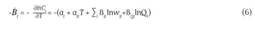
where the basic assumption is that costs decrease due to technology improvements. a t is the constant rate of technical change, a tt T captures variations in the rate of technical change over time, ∑ i ß it lnw it is the input bias and ß Qt lnQ t is the scale bias. Therefore, pure technical change is equal to -(a t + a tt T), which corresponds to the rate of reduction in overall costs due to a technical innovation, holding constant the scale effect. Also, scale augmenting technical change is measured by -ßQ t lnQ t , which is the rate of reduction in costs due to a technical innovation exhibited along with changes in output. Similarly, biased technical change (IBTC) was computed using the following expression when the production function behind a translog cost function is non-homothetic (Antle and Capalbo, 1988):

where  captures the potential biased technical change exhibited by the input i and
 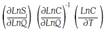 denotes the scale effect of technical change. These results can be used to test the presence of biased technical change, which can be described in terms of input-saving or using, which indicates the rate of change in cost shares due to technical change,
  and is a relative concept. That is, input saving means that the ratio of the input relative to others is declining rather than the absolute quantity of use of the input declining, although it is possible for both to occur simultaneously.
Finally, agricultural productivity growth (TḞP) in this model is measured using equation (8):

where  is the shift estimated for the cost function due to technical change and
  is equal to
 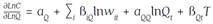 (Capalbo, 1988). This approach was also used to individually estimate crop and livestock productivity.
4.4 Structural Change Periods
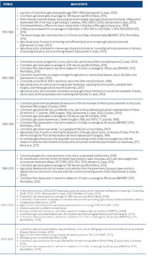
Historical evidence suggests that Colombia’s agriculture faced substantial and distinct structural changes over time (see Table 1). Accordingly, six periods of changing economic conditions and policy regimes were analyzed in an effort to determine whether or not Colombia’s agricultural productivity and technical change were affected. These periods were identified by conducting a historical analysis of Colombia’s agriculture from 1975-2013. Each period was defined based on: i) macroeconomic issues; ii) political changes; iii) economic policy changes (e.g. trade policy); and iv) socioeconomic issues, such as violence.16 These impacts on agricultural productivity were estimated by including six period specific time trend variables in the Cobb-Douglas regressions. Also, a comparison of the predicted output with and without technical progress was made for the CES and Translog Cost functions.
Table 1 Main Events Determining Colombia’s Agriculture from 1975-2013 17
| Period | Main Event |
| 1975-1983 | Coffee boom |
| 1984-1989 | Macroeconomic crisis |
| 1990-1997 | Agricultural profitability crisis |
| 1998-2002 | Armed conflict intensification |
| 2003-2009 | Agricultural commodities price boom |
| 2010-2013 | Agricultural profitability crisis |
5. Data
The underlying data used in this study primarily come from FAOSTAT, the World Bank and the USDA (FAO, 2015; USDA, 2015; World Bank, 2016). In order to expand the data available for Colombia, recent data from the National Department of Statistics of Colombia (DANE), the Central Bank of Colombia (BANREP) and the International Fertilizer Industry Association (IFA) were used (BANREP, 2015; DANE, 2015; IFA, 2016). A historical database for Colombia’s’ agriculture from 1975-2013 was built based on these data sources. This database includes the value of Colombia’s agricultural output (aggregated and disaggregated by crops and livestock) and quantities as well as the prices of inputs (labor, capital, fertilizer and animal feed). An estimation of some of these data series was necessary to focus the analysis on these four inputs, given the problems of data availability for all available sources and the time period analyzed in this paper. The construction of each variable is explained in detail below.
5.1 Output
The value of agricultural production corresponds to the total gross production value released annually by FAOSTAT (FAO, 2015).18 In the case of Colombia, this figure encompasses the value of production for 85 crops and livestock commodities.19 These data were used as they were released annually (per calendar year) and in 2005 international dollars. FAOSTAT releases these data in this currency unit in order to facilitate comparisons across countries. The aim is to avoid the need to use exchange rates by assigning a single global price to each commodity.
For crops, the data correspond to the crop category as reported by FAOSTAT. This includes data for 74 crops produced in Colombia, sold in the market, and consumed by consumers. These figures were multiplied by producer prices and converted to 2005 international dollars (FAO, 2015). For livestock, the data source is FAOSTAT as well and corresponds to its livestock category, including the production of eleven animal products (cattle meat, poultry meat, pork meat, milk, etc.) multiplied by producer prices.
5.2 Inputs
5.2.1 Capital Stock
The capital stock data corresponds to Colombia’s gross capital stock used in agriculture and released annually by FAOSTAT (FAO, 2015). This is calculated as the sum of valued individual physical assets held by Colombian farmers (FAO, 2015). This dataset includes separate data for land development (i.e. arable land, crop land, and irrigated land), plantation crop land, livestock (i.e. fixed assets and inventory), machinery and livestock structures.
Crop capital stock compiles the value of gross capital in plantation crops and land development (FAO, 2015).20 Livestock capital stock encompasses the value of livestock fixed assets, livestock inventory and livestock structures. FAO also releases figures for capital stock in machinery and equipment (FAO, 2015). However, these figures include assets that can be owned by either activity, such as tractors. Accordingly, this stock was divided for crops and livestock using their respective overall shares in the total value of agricultural production.
Capital stock data in FAOSTAT is only available from 1961-2007. Consequently, this data series was updated for more recent years based on the gross investment flows to Colombia’s agriculture from DANE (2015).21 The data was used as it is released annually (per calendar year) and in 2005 dollars.
The cost (input price) of capital was also estimated by relying on the definition of cost benefit analysis. This considers the cost of capital as the opportunity cost of investing in a particular asset (Campbell and Brown, 2003). Therefore, its measurement corresponds to the sum of the real interest rate plus the depreciation rate of agricultural assets. The real interest rate is calculated as the difference between the nominal interest rate and current inflation rate. This nominal interest rate corresponds to a traditional passive interest rate in Colombia, also known as DTF (i.e. the Fixed Term Deposit Rate in Colombia) because there is not an official interest rate for agricultural credit in Colombia and loans for agriculture are often indexed to this interest rate. In addition, agricultural credits are often subject to a subsidy according to the type of farmer (i.e. small, medium or large), which (for this paper and other research) corresponds to a deduction of 5 percentage points from this interest rate (Illera, 2009; Jaramillo and Jiménez, 2008).22 Finally, the depreciation rate for agriculture was taken from Pombo (1999), who calculated the average depreciation rates exhibited by capital for all economic activity in Colombia. The current inflation rate was taken from the World Bank (2016).
5.2.2 Labor and Wages
The farm labor data used in this paper corresponds to the total number of people who were economically active in Colombia’s agriculture, as released by the USDA from 1961-2012 (USDA, 2015). An update was conducted for the last decade (2001-2013) using available data from national sources (DANE, 2015). Annual data were used as they were released (per calendar year).
Crops and livestock data were estimated based on Barrientos and Castrillón (2007), whose study analyzes the employment generation path of Colombia’s agriculture and shows disaggregated labor data for Colombia from 1993-2005. These data were used as a starting point to estimate the missing labor data for the sample period. It was necessary to estimate labor data for crops and livestock from 1975-1992 and 2006-2013. For this purpose, the average trend of the labor data over time within the sample was used in each case, for which crops exhibited an R2 of 0.98 and livestock an R2 of 0.72.23 These estimates were then adjusted using the aggregate labor data collected from the USDA (USDA, 2015). This involved the estimation of weights for crop and livestock labor in the total predicted data, followed by the multiplication of these weights by the USDA’s aggregate agricultural labor data. The process ensured that these predicted labor data for crops and livestock were consistent with the USDA data.
Farm labor wages were implicitly derived from annual national accounts (DANE, 2015). That data revealed the total payroll of each Colombian sector to generate sectoral GDP. Thus, the value paid to labor by agriculture was taken in current pesos, and an estimated average wage paid per employee was calculated by dividing this figure by total farm labor. The amount was then converted into 2005 dollars by: i) dividing this value by the annual average Colombian exchange rate of peso to US American dollars (BANREP, 2015); and ii) dividing the result by the GDP deflator for US prices with the base year of 2005 (FAO, 2015).24
5.2.3 Fertilizer
Fertilizer quantities correspond to the total amount of major nutrients (N+P2O5+K2O) demanded and applied by farmers in Colombia, released yearly by the IFA (2016). These data include all compound products derived from nitrogen (N), phosphate (P) and potash (K), such as Urea, Ammonium Sulphate, Ammonium Nitrate, Ammonium Phosphate and Potassium Sulphate, among others. Annual data were used as released per calendar year and in metric tons.
Fertilizer prices in Colombia were estimated based on FAOSTAT, DANE and BANREP data (BANREP, 2015; FAO, 2015; DANE, 2015). There is no available historical database that compiles these prices for Colombia for the entire period covered by this study (1975-2013). The available data is only for more recent years (AGRONET, 2014). An estimation of earlier fertilizer prices was completed using the urea price paid in Colombia by farmers as a leader-indicator or benchmark price.25 This price was reported annually (per calendar year) by FAOSTAT in current Colombian pesos per metric ton for the period 1961-2002. However, the data exhibits some missing values for the 1990s, which this paper approximated using the annual change in the Producer Price Index (PPI), released by BANREP since the early 1990s and by DANE in recent years (BANREP, 2015; DANE, 2015).
5.2.4 Animal Feed
Animal feed quantities used in this paper come from FAOSTAT (FAO, 2015) and correspond to the total crop and animal products used for feeding animals following the USDA (2015). FAOSTAT reports these quantities in its Commodities Balance Sheet. These annual data were used as they were released per calendar year and in metric tons.
The animal feed price was derived from FAOSTAT (FAO, 2015). Basically, this price was implicitly estimated as a weighted average. The producer prices of crop and animal products used for feeding animals reported by FAOSTAT were taken, and the value of each feed was calculated using their quantities. Then, the total annual value was calculated for these products. Finally, this total value was divided by the total product quantity to calculate an average price per metric ton of animal feed for each year. Because this figure was in current Colombian pesos, it was then converted to 2005 dollars.
6. Results
Using the three techniques discussed in Section 4, we obtained the necessary parameters to measure Colombia’s agricultural productivity growth from 1975-2013. Table 2 presents the results using a Cobb-Douglas production function. Table 3 presents the results of the CES function.26 27 Tables 4 and 5 present results from the Translog Cost function approach and the own price elasticities for all inputs to evaluate the estimated cost function.28 29 Overall, the Cobb-Douglas results clearly show statistically significant evidence that Colombia’s technical change exhibited different trends during each period defined a priori (see Table 2). This varied between 0.5-0.9% per year across periods. These structural changes were not incorporated when estimating the CES production function and Translog Cost approach due to insufficient degrees of freedom. Thus, the results represent an average over the different regimes. However, a comparison of the agricultural productivity growth trajectories predicted by these approaches using a Cobb-Douglas production indicates that all follow almost the same pattern (see Figure 1). Moreover, the CES results show the presence of biased technical change in Colombia’s agriculture, and the Translog Cost approach results highlight an important contribution of scale effects into Colombian agricultural productivity.30
In the next section, all estimates found using each technique are analyzed with emphasis on three modes of inquiry: i) What was Colombia’s agricultural productivity growth-aggregated and also disaggregated for crops and livestock-during this entire period? ii) Did Colombia’s agricultural productivity vary during sub-periods when particular economic conditions or policy regime changes were identified?; and iii) Did Colombia’s agriculture exhibit biased technical change during the period 1975-2013?
Table 2. Cobb-Douglas Production Function Estimates for Colombia’s Agriculture from 1975-2013
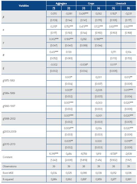
Robust standard errors in parentheses
* p<0.10, ** p<0.05, *** p<0.01
Models assuming constant technical change are: (1), (3) and (5)
Models assuming technical change by structural change period (see Table 1) are: (2), (4) and (6)
ß is the coefficient of lnLt (Labor)
a is the coefficient of lnKt (Capital)
γ is the coefficient of lnFt (Fertilizer)
θ is the coefficient of lnSt (Animal Feed) g is the rate of technical change
Table 3 CES Production Function Estimates for Colombia’s Agriculture from 1975-2013
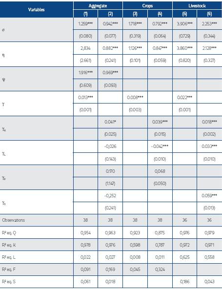
Robust standard errors in parentheses
* p<0.10, ** p<0.05, *** p<0.01
Models assuming Hicks-Neutral technical change are: (1), (3) and (5) Models assuming bias technical change are: (2), (4) and (6)
σ is the overall elasticity of substitution between nests
η and ψ are the elasticities of substitution of inputs within each nest
γ is the overall rate of technical change
γi is the rate of technical change exhibited by a particular input
Table 4 Trans-Log Cost Function Estimates for Colombia’s Agriculture from 1975-2013
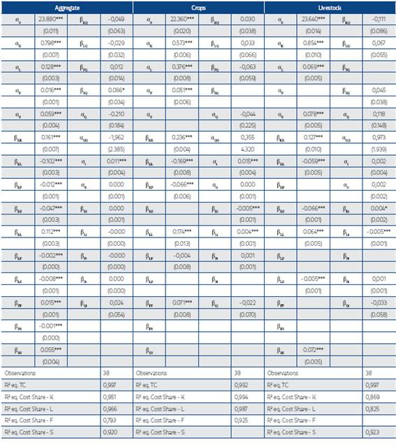
Robust standard errors in parentheses
* p<0.10, ** p<0.05, *** p<0.01
αi are the cost shares at the point of approximation of the cost function
βij are the elasticities of cost shares with respect to input prices
βiQ are the elasticities of cost shares with respect to output
αt, αtt and βit are the elasticities of cost function and cost shares relatively with respect to technical change
Table 5 Price Elasticities of Input Demands of the Trans-Log Cost
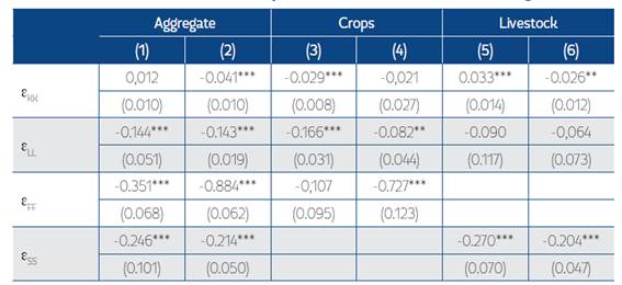
Standard errors in parentheses
* p<0.10, ** p<0.05, *** p<0.01
Without imposing curvature restriction: (1), (3) and (5)
Imposing curvature restriction: (2), (4) and (5)
6.1 Colombia’s Agricultural productivity
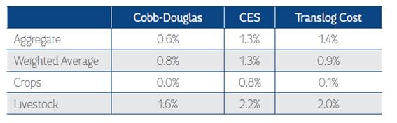
These results show that Colombia’s agricultural productivity grew on average 0.6-1.4% from 1975 to 2013 (see Table 6). In particular, the CES and Translog Cost techniques predict that it grew on average around 1.3-1.4% per year, respectively, which is similar to the USDA’s prediction (1.4%). The Cobb-Douglas technique predicts that Colombia’s agricultural productivity only grew by 0.6% per year.
These predictions of Colombia’s agricultural productivity were estimated using aggregate data. Although all looked very similar, some key differences were identified. Accordingly, we estimated Colombia’s agricultural productivity using disaggregated data for crop and livestock productivity. This approach renders more consistent predictions for Colombia’s agricultural productivity and removes any difference across techniques generated by the use of aggregate data. Hence, we estimated Colombia’s agricultural productivity as a weighted average of the estimates of crop and livestock productivity, using the shares of crop and livestock production values as weights in total agricultural production value.
This exercise shows that the initial estimates for Colombia’s agricultural productivity using aggregate data maybe slightly overestimated or underestimated. Using Cobb-Douglas techniques, the initial prediction was that productivity has grown by 0.6%; however, it grew by 0.8% per year when computed as the weighted sum of crop and livestock productivity. Likewise, using Translog Cost model, the prediction was that the productivity average growth was around 1.4% per year, but it grew by 0.9% per year when estimated as the weighted sum of crop and livestock estimates. Only the CES technique provided similar estimates regardless of approach. This exercise reaffirmed our initial estimates using aggregate data, showing that Colombia’s agricultural productivity exhibited very low growth from 1975-2013. Also, it suggests that productivity grew in a narrower range, between 0.8% and 1.3%, once a more nuanced crop and livestock productivity performance was considered. These weighted average estimates for Colombia’s agricultural productivity are used in the rest of our analysis.
These estimates show that livestock productivity was the driver of Colombia’s agricultural productivity from 1975 to 2013. All techniques predict that livestock productivity grew at an average rate between 1.6% and 2.2%, probably due to: i) more efficient production practices in the pork and poultry sectors; ii) higher investments in new herds and technology (mainly dual-purpose cattle) in the late 1990s; and iii) innovations for the feeding and management of livestock, genetic improvements and the purchase of highly productive species in the milk sector (Kalmanovitz and López, 2003; MADR, 2005; Mojica and Paredes, 2005). It is not inconsequential that the poultry and pork sectors of Colombia were dominated by completely vertically-integrated, large-scale producers. These entities have brought modern production systems, improved feeding strategies and advanced the breeding and veterinarian expertise of the animal sector.
Colombia’s crop sectors, with the exception of sugar cane and rice, were dominated by small-scale production, a lack of access to improved technology and potential market power by multinational buyers. The latter is especially true for Colombia’s most famous crop, coffee, for which the benefits of advances in world demand have mostly accrued for multinational processors and retailers, and thus have not led to productivity gains in agricultural production. Also, investments made to replace rust-susceptible coffee trees with rust-resistant trees have required agricultural inputs such as labor and nursery stock, which will not yield significant or immediate productivity gains. These latter investments began to generate productivity enhancements in 2016-2017 (USDA, 2017).
Predictably, the estimates of crop productivity are unclear for this period. Assuming a Cobb- Douglas production function and using the Translog Cost approach, the prediction is that Colombia’s crop productivity’s average growth was zero. However, when assuming a CES production function, crop productivity grew on average by 0.8% per year, which is still low.
Historical evidence suggests that crop productivity would have been low during the period 1975- 2013. Colombian farmers experienced difficult conditions during this period due to: i) agricultural budget cuts during the 1980s Latin American debt crisis; ii) profitability crisis after Colombia executed the second wave of Structural Adjustment reforms in the early 1990s; iii) extreme weather conditions (i.e. severe droughts and severe floods); iv) misallocation of resources for agricultural promotion; v) decreased investment due to armed conflict; vi) lack of public resources for promoting Colombia’s agricultural competitiveness and vii) segmented and restricted funding of Colombian farmers (Cuevas et al., 2003; Jaramillo, 1998; Junguito, 1994; Junguito et al., 2014; Kalmanovitz and López, 2003; Reina et al., 2011). Also, this evidence suggests that only a few crops exhibited higher levels of productivity during this period (e.g., sugar cane, flower, banana, cereals and vegetables) (Arbeláez, 1993; Becerra, 2009; COMPITE, 2008; Jaramillo, 1998; Montero and Casas, 2012; Ramirez and Garcia, 2006).
In order to reaffirm these findings, we tested the consistency of these annual estimates of Colombia’s agricultural productivity growth across techniques. First, we conducted a graphical analysis of Colombia’s estimated agricultural productivity trends. This figure clearly shows that all techniques predict similar patterns of Colombia’s agricultural productivity during the period 1975-2013 (see Figure 1). Furthermore, this analysis indicates that these estimates exhibit practically the same turning points; the only difference is the magnitude of certain periods of growth or depletion (see Figure 1).
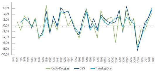
Second, we calculated a correlation matrix using the annual predictions of Colombia’s agricultural productivity for each technique from 1975-2013. Overall, this correlation varied between 70% to 95%. The highest correlation is between the agricultural productivity predicted by assuming a CES production function and the Translog Cost approach (+94%), whereas the lowest correlation is between the agricultural productivity predicted by assuming a Cobb-Douglas production function and the Translog Cost approach (73%) (see Table 7). These results reaffirm that there is a high consistency across all estimates and techniques used in this study. Also, all techniques broadly predicted similar results for Colombia’s agricultural productivity over time.
6.2 Components of Colombia’s Agricultural Growth
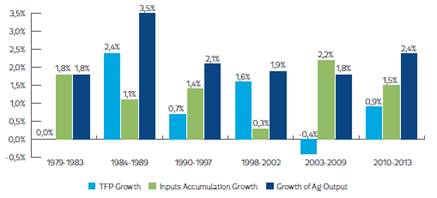
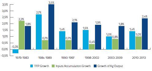
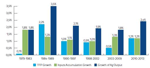
Given the high consistency of these estimates for Colombia’s agricultural productivity, our subsequent analysis focused on examining the possible drivers of Colombia’s agricultural growth during the period 1979-2013: agricultural productivity growth or input accumulation growth. To this end, we considered the six periods previously defined, during which: i) Colombia’s agriculture exhibited similar economic conditions and ii) agricultural policy regimes did not drastically change (see Table 1).
Using the predictions of Colombia’s agricultural productivity by technique, we found that Colombia’s agricultural production growth exceeded 2% per year whenever agricultural productivity growth increased (e.g. in the late 1980s and in recent years; see Figures 2, 3 and 4). These estimates suggest that Colombia’s agriculture only grew by 1.8% per year from 1979 to 1983 due to an agricultural productivity growth close to 0%, largely explained by the negative impact of the Latin American Debt crisis on Colombian agriculture (Kalmanovitz & López, 2003). From 1984-1989, the agricultural output value increased its average growth to 3.5% per year, the effect of higher agricultural productivity, which grew around 2.2-2.7% per year due to the following favorable conditions: i) agricultural policy focused on promoting private investment, adjusting the price system, raising farmer’s margins, limiting agricultural imports, etc.; ii) higher commodity prices; and iii) productivity innovations carried out by farmers to overcome the early 1980s crisis (Guterman, 2007; IMF, 2015; Kalmanovitz & López, 2003; Reina et al., 2011). During the period 1990-1997, Colombia’s agriculture exhibited a slowdown and grew on average by 2.1% per year. Annual productivity grew on average only by 0.7-1.4%, seemingly due to the severe profitability crisis exhibited by Colombia’s agriculture during this period. From 1998-2002, Colombia’s agricultural output slightly reduced its growth to 1.9% per year because: i) agricultural productivity stagnated to 0.9-1.6% growth per year; and ii) farmers diminished their input accumulation, probably due to the macroeconomic crisis and worsening armed conflict during this period. Over 2003 to 2009, Colombia’s agriculture continued stagnating, growing at the pace of the 1990s due to a slower agricultural productivity growth (-0.4-1%) caused by: i) lack of political agreement on how resources should be allocated to support agriculture; ii) poor transportation infrastructure; and iii) lack of innovation and technological development to improve agricultural productivity (Reina et al., 2011). Finally, we found that Colombia’s agriculture raised its average growth to 2.4% per year from 2010-2013, due to an increased agricultural productivity growth of 0.9-1.4% per year. In other words, Colombia’s agricultural growth has been less sensitive to input accumulation and more sensitive to productivity trends, policy regimes and economic circumstances.
6.3 Biased Technical Change
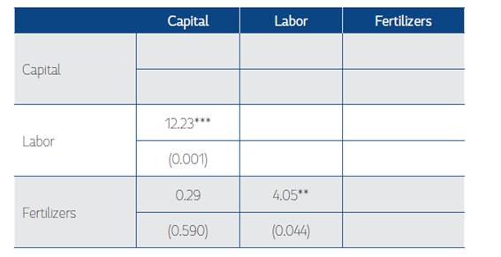
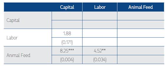
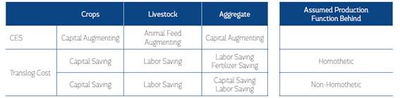
All estimates show that Colombia’s agriculture exhibited biased technical change during the period 1975-2013 (see Table 10). The CES results show that technical change was capital augmenting using data for the entirety of Colombia’s agriculture. The technical change exhibited by capital grew on average by 4.1% per year over this period, whereas the technical change exhibited by other inputs was not statistically significant (see Table 3). We also found that the technical change in crop production was capital augmenting. The difference across the technical change coefficients estimated for each input was tested because some were statistically significant. There is a statistically significant difference between the technical change exhibited by capital and labor as well as the technical change coefficients exhibited by fertilizer and labor (see Table 8). However, there is no statistical difference between the technical change coefficients found for capital and fertilizer. Likewise, we found that livestock production was animal feed augmenting. We also tested these differences across coefficients, and there is a statistically significant difference between the technical change exhibited by animal feed relative to the technical change exhibited by capital and labor (see Table 9). Also, we found that there is no statistically significant difference between the technical changes exhibited by capital and labor in livestock production.
Table 8 Test of Differences among Technical Change Estimates Exhibited by Inputs in Crop Production
P - values in parentheses
*This is a symmetric matrix.
*** p<0.01, ** p<0.05, * p<0.1
Table 9 Test of Differences among Technical Change Estimates Exhibited by Inputs in Livestock Production
P - values in parentheses
*This is a symmetric matrix.
*** p<0.01, ** p<0.05, * p<0.1
Translog Cost estimates reaffirm these results for crops, showing that crop production was capital saving. However, the cost model results suggest that livestock production was labor saving.31 The statistical difference across these technical change indices was not tested, because multicollinearity is a latent problem when a Trans-Log cost function is assumed (Christensen and Greene, 1976). Thus, the standard errors for all parameters may be larger and this test would yield untrustworthy results. Consequently, this analysis only involved a comparison of the magnitudes across these indices.
In any case, the CES and Translog Cost results indicate that changes in the input efficiency of Colombia’s agriculture varied across agricultural activities during 1975-2013. Also, technical change tended to improve the marginal productivity of capital in crop production, and marginal productivity of animal feed and labor in livestock production more so than the marginal productivity exhibited by other inputs.
7. Conclusions
This paper measured Colombia’s agricultural productivity from 1975-2013. Using three different econometric specifications, it found evidence that it grew on average between 0.8% and 1.3% per year. All methods used in this study-Cobb-Douglas production function, CES production function and Translog Cost function-estimate that Colombia’s agricultural productivity was mainly driven by livestock productivity, which grew on average between 1.6% and 2.2% per year. It is likely this growth was driven by improved technologies and the input quality enhancements of larger vertically-integrated poultry and non-ruminant producers. In contrast, crop productivity expansion is unclear over this period. By assuming a Cobb-Douglas production function and using the Translog Cost approach, it is predicted that crop productivity growth was zero; by assuming a CES production function, it is predicted that crop productivity grew on average by 0.8% per year.
This paper also finds evidence that agricultural productivity was a crucial factor of agricultural production value growth in Colombia in recent decades, especially during periods of sustained growth. Agricultural production growth accelerated to more than 2% per year when agricultural productivity growth increased (e.g. in the late 1980s and in recent years). Moreover, all results suggest that the pace of agricultural productivity was strongly dependent on policy regimes and economic circumstances. Recent peace initiatives should enable improved political and economic circumstances conducive to more rapid economic growth. That being said, better livelihoods for those returning to rural activities require supportive polices that foster long-term productivity rather than the short- term infusion of inputs. Thus, Colombia’s agricultural policy must prioritize productivity, a crucial determinant of agricultural growth. Policies that focus on access to improved practices, credit, and efforts to enhance human capital development (i.e. education and healthcare) should be high on the government’s list for rural development.
Finally, this study finds evidence that Colombia’s agriculture exhibited biased technical change during the period 1975-2013. The results indicate that technical change tended to improve the marginal productivity of capital in crop production and the marginal productivity of animal feed and labor in livestock production relative to other input categories. Scale effects also mattered to productivity growth when the Translog cost function method that permits the identification of such effects was employed. While the more advanced techniques did not exhibit significantly different overall productivity estimates over time, they did enable the examination of these more nuanced aspects of productivity growth.
Future studies might conduct similar analyses on that sectoral level. Colombia is a country that produces a wide variety of agricultural products, and each agricultural sector uses different production structures and key input ratios. Hence, measuring and analyzing productivity on the sector level is key to understanding which microeconomic forces drive the results of this paper. Furthermore, future studies have the potential to improve Colombia’s agricultural policy by identifying its most influential sectors. In order to conduct such studies with sufficient accuracy, data collection investments are necessary.