


 Inglés (pdf)
 Articulo en XML
 Referencias del artículo
 Enviar articulo por email
 Citado por SciELO
  Citado por Google
  Similares en
SciELO
Similares en
SciELO  Similares en Google
 Permalink
Introduction
Developed economies have shown a sluggish recovery after the 2008-2009 crisis. First, they set historically low monetary policy rates (such as the effective federal fund rates of the United States, which was below 0,25 % between 2009 and 2015), significantly limiting the policy scope. The commodity prices were also at relatively low levels; therefore, less sensitive to adjustments. Then, the total world trade contracted more than 7 % on average during 2015-2016, followed by a gradual recovery pace that turned back during 2018. This scenario occurred in a context with significant debt accumulation and a low propensity for real investment (Prat and Solera, 2017). This behavior might reveal the onset of structural lower aggregate demand and reduced recovery capacity, raising doubts about the growth prospects worldwide. So a couple of issues emerge: Was there a pre-pandemic slowdown? Are we facing secular stagnation?1
This paper aims at understanding whether the economic growth of Central America2 and the Dominican Republic (CADR) was compromised before the 2020 pandemic. Looking for robustness, I apply different statistical and structural methodologies to estimate the potential growth of these countries, shedding light on its pattern over time to verify if the actual growth was deviating from its potential more than before. As mentioned by Manzano and Maldonado (2016), CADR countries not only had to deal with the 2008-2009 crisis but they have also been suffering external shocks during the last decades, significantly increasing their macroeconomic vulnerability. They are small economies, highly dependent on foreign trade, and, in most cases, remittances. Figure 1 shows the average real growth of CADR since the sixties, while Figure 2 indicates how these countries depend on the international scenario. The context makes it difficult to rule out a slowdown in the region even before the pandemic.
In this field, a new normal describes a constant state of weak demand with few and unusual episodes of full employment, a context in which countries might reach a lower potential growth rate than before or even a negative natural rate. It is understood not only as of the need for having negative real interest rates to equal out savings with investment under full employment but as the difficulty of achieving financial stability and a high potential growth rate through conventional monetary policy.
This setup centered its attention on developed countries, as drivers of global economic effects, and comes up recently as a topic for debate (Summers, 2013 and 2014; Krugman, 2014; Fernald, 2015; Bernanke, 2015a and 2015b; Eichengreen, 2015; Gordon, 2015; Caballero and Farhi, 2018; Di Bucchianico, 2020). Nevertheless, the inherent dynamics of emerging countries and their remarkable dependence on external factors makes it possible to consider it a worldwide phenomenon.
CADR has boasted a higher growth rate than the rest of Latin America. In 2015, they had favorable expectations based on both the slow but gradual recovery of the United States (leading trading partner) and better terms of trade with low oil prices.3 However, this favorable context was not fully recognized and is now changing. The Federal Reserve of the United States gradually increased its interest rates from ultra-low (near zero) to historically normal levels. At the same time, the oil prices showed signs of recovery during 2016 and most of 2018. Also, developed countries seem to be facing weak demand and less historical growth, a macroeconomic situation deepened by the recent pandemic (Davies, 2020).
The potential growth is an unobserved variable; thus, there is no precise method to estimate it. Miller (2003) reminds us that particular characteristics feature each country, and each method has its advantages and disadvantages, lending uncertainty to these estimations. One way to deal with this concern is to follow different approaches (Cotis, Elmeskov, and Mourougane, 2004). Looking for robustness and using annual data, I herein estimate the potential growth of CADR countries using two main approaches:
Statistical, with full/recurrent use of statistical tools or filters. Three methods are applied: i) Hodrick- Prescott filter (HP) by constrained minimization, following both the variability of the acceleration of the trend relative to the variability of cyclical component, and the variability of the acceleration in the trend component; ii) Production function (PF), using a standard Cobb-Douglas with skill-adjusted labor (human capital); and, iii) Regime-switching model (SM) based on three growth scenarios: recession or moderate, sustainable, and overheated.
Structural, using a Bayesian model averaging over panel data to produce robust country-structure variable specifications and test the significance of country effects on the pre-pandemic period. This process is based on several variables falling into six categories: growth theories (usually considered in theoretical models); convergence; educational system; economic openness; institutional quality; and economic structure.
The contribution of this paper is threefold. Firstly, CADR countries have no recent estimations of potential growth and output gaps using historical data and following different methodologies throughout statistical and structural approaches. Johnson (2013) comes up with an applied effort estimating potential output for these countries, but only using production function, switching, and state-space methods. Also, Johnson (2013) excludes Belize from the sample and does not consider historical data. Besides, in this paper, I use an unbalanced panel with 39 high-income, 52 medium- income, and 11 low-income countries, as well as 40 variables to test robust determinants of potential growth using a Bayesian model averaging. This panel differs from studies such as Lanzafame et al. (2016), in which at most 70 countries are included (leaving aside most of the Central American countries) considering 34 possible determinants. The use of different methodologies allows to gain robustness and widen the analysis of potential growth. In fact, contrasting all the outputs, this paper confirms that statistical models show a higher potential growth for CADR countries, signaling that the region would be closer to structural growth in a less favorable context.
Secondly, this analysis allows us to verify if particularities might be structurally limiting potential growth. Following structural models, I confirm the presence of country-specific vulnerabilities and find positive and negative fixed effects statistically significant for each country of CADR, revealing a scenario not only featured by exogenous factors but by individual results. Nevertheless, this approach faces at least one limitation, it accounts for particularities and allows to conclude their presence, but it does not identify the specific determinants and constraints per country that might be causing dissimilarities. In this sense, exploring and identifying heterogeneities in potential growth drivers could be valuable for further research.
Thirdly, this paper is an applied effort to understand better the vulnerability of the economic growth of CADR countries before the global pandemic shock. Moreover, I identify an aggregate slowdown experienced by CADR before the shock, with mixed country results. Most countries show a relative deacceleration of observed and potential growth and pre-pandemic macroeconomic conditions hindering their recent shock response. This situation deserves to be highlighted. The economic impacts of the pandemic on the region might be deepening the already aggregate slowdown of the potential growth.
This paper is organized as follows: In the next section, I describe each of the statistical methods; the third section exposes the Bayesian model averaging approach; the fourth section reviews the main results; and the fifth section comprises the conclusions.
2. Statistical Approaches
This section focuses on describing the methodologies that use full/recurrent statistical tools over annual data for each country.4
2.1 Hodrick-Prescott Filter by Constrained Minimization.
The HP filter decomposes a time series (y t ) into a trend (y t ) and a cyclical component. The sum of squared deviations from the series’ trend is minimized, penalizing changes in its acceleration through a smoothing parameter λ. Equation (1) shows the conventional HP filter.
 (1)
(1)
This filter involves a clear problem: arbitrariness in the selection of λ. The value depends on the frequency of the series. Researchers usually adopt Hodrick and Prescott’s setup (in their 1980 analysis on the United States), that is, to use λ=100 for annual data, λ=1600 for quarterly data, and λ=14400 for monthly data. Nevertheless, the properties of economic cycles differ among countries. Hence, the use of such values does not guarantee reliable and consistent results. As an alternative, I follow two assumptions from Marcet and Ravn (2004) to calculate two optimal λ by country, making them comparable with the traditional standard values. In this case, Equation (2) identifies the objective function to minimize:
 (2)
(2)
Firstly, I assume larger variability of the growth rate in countries with a more volatile cyclical component (some countries might have larger deviations from a linear trend than others). This procedure (also called V methodology) considers the variability of the acceleration of the trend relative to the variability of the cyclical component. The idea is to minimize Equation (1) subject to Equation (3) in which the relative variability must be at most equal to a positive constant V:
 (3)
(3)
Secondly, the trend’s growth might have the same variability across countries (similar deviation between the actual trend and a linear trend). Therefore, this procedure (also called W methodology) focuses on the variability of the acceleration in the trend component of each country. In this case, Equation (1) is minimized subject to Equation (4), where the variability of the acceleration trend adjusted by T-2 observations is limited at the top by a positive constant W:
 (4)
(4)
V and W are not chosen arbitrarily, I calculate the components of the standard HP filter as calculated for the United States and the respective restrictions. In this sense, the results are conditional to the United States scenario (λ=100) as sample reference but country-specific in the output. I apply the filter to the real GDP logarithm with those parameters and its differences approximate the potential growth. By restriction, Table 1 presents the results of the optimal λ.
Table 1 Optimal Smoothing Parameter
| Optimal λ | Belize | Costa Rica | Dominican Republic | El Salvador | Guatemala | Honduras | Nicaragua | Panama |
| V | 152 | 143 | 108 | 226 | 247 | 100 | 191 | 120 |
| W | 740 | 260 | 420 | 1500 | 420 | 58.5 | 8857 | 740 |
Using these parameters would have the immediate advantage of better-adjusted calculations, and they represent new reference values for future research for CADR countries.
The data comes from Penn World Table 9.0 (PWT) and the World Economic Outlook (International Monetary Fund, April 2018). The latter allows us to extend the final range of the series to 2023, reducing the bias generated by sample endpoints, where the cycle component is underestimated.
2.2 Production Function.
Following Sosa, Tsounta, and Kim (2013) I assume a standard Cobb-Douglas production function with skill-adjusted labor (human capital) and constant returns to scale for each country, as in Equation (5):
 (5)
(5)
The real output (Y t ) is determined by the technological progress (A t , calculated as residual), a capital factor (K t ), and a labor factor (L t ) skill-adjusted by a human capital index (h t ). In this case, α t is a country-specific output elasticity to capital (averaging the values from PWT 9.0).
The capital factor is calculated in two stages, assuming an economy with balanced growth in t=0, the initial value of the capital factor (T 0) comes from Equation (6):
 (6)
(6)
I 0 is the average weight of real investment over GDP from t=0 to t=4 multiplied by the initial GDP, minimizing the impact of future fluctuations. The parameters are the following: the technological progress growth (g) is a constant for all countries that equals 1,53 % (assumed by Ferreira, Pessôa, and Veloso 2012, in their analysis about the evolution of total factor productivity in Latin America); the population growth rate (n) is country-specific, averaging the sample growth rate of the population until 2014 and assuming medium-fertility variant of the population in 2015-2023 (taken from the United Nations World Population Prospects); and a time-varying depreciation rate (δ t ) from PWT 9.0.
For K t , where t>0, I consider the perpetual inventory method to approximate capital stock at full capacity (Equation (7)):
 (7)
(7)
The labor factor is measured on the basis of the number of workers. Following Bils and Klenow (2000), h t is calculated as in Equation (8). In this case, Barro and Lee (2013) have estimations of the total years of schooling (s, using linear interpolation whenever missing values). The parameters θ and ψ equal 0.188 and 0.368, respectively (Fernández-Arias, 2014).
 (8)
(8)
Finally, the potential real GDP is obtained from Equation (9), that is, calculating the exponential values of the linearized function. Except for the capital, each factor represents the respective trends using the standard HP filter.5
 (9)
(9)
2.3. Regime-Switching.
The real GDP growth rate might have experienced significant breaks while moving across different growth paths or regimes. In this case, three growth regimes are taken into account: recession (or moderate growth), sustainable (potential path), overheated. No permanent shocks are considered, which means that neither recession nor economic over-heating represents an absorbing state.
The regime-switching model follows an iterative procedure. A set of stationary processes (stable variance-covariance matrix), represented with different probability density functions, generates a time series (y t ), allowing variability on a given number of scenarios.6 Then, an expectation-maximization (EM) algorithm is applied to find the most likely estimators of parameters.7 ∀ scenario = j =1,2,3, this procedure is carried out through Equations (10), (11) and (12):
Estimated growth (θj):
 (10)
(10)
Estimated volatility (σj 2)
 (11)
(11)
Unconditional probability (πj):
 (12)
(12)
With  variable generated from the distribution function is s
t
, the number of iterations is k, and Γ is the parameter vector (set of conditional information). Table 2 shows the outcomes for each scenario in our unbalanced panel.
variable generated from the distribution function is s
t
, the number of iterations is k, and Γ is the parameter vector (set of conditional information). Table 2 shows the outcomes for each scenario in our unbalanced panel.
Table 2 Convergence Results (%)
| Countr y | Growth | Growth | Growth | Standard Deviations | Standard Deviations | Standard Deviations | Unconditional Probability | Unconditional Probability | Unconditional Probability |
| Recession or Moderate | Sustainable | Overheating | Recession or Moderate | Sustainable | Overheating | Recession or Moderate | Sustainable | Overheating | |
| Belize | 2.2 | 4.9 | 9.2 | 1.8 | 0.2 | 2.5 | 60.2 | 20.0 | 19.9 |
| Costa Rica | 2.3 | 4.9 | 7.9 | 5.4 | 2.5 | 5.1 | 10.7 | 77.3 | 12.0 |
| Dominican Republic | -7.9 | 5.4 | 18.0 | 3.3 | 3.4 | 0.5 | 2.5 | 94.7 | 2.8 |
| El Salvador | -6.1 | 2.1 | 4.4 | 2.5 | 0.3 | 2.4 | 5.8 | 29.9 | 64.4 |
| Guatemala | 2.2 | 3.9 | 7.5 | 2.8 | 0.9 | 1.4 | 25.6 | 62.9 | 11.5 |
| Honduras | -1.1 | 4.2 | 4.9 | 3.6 | 1.6 | 0.8 | 12.6 | 67.5 | 20.0 |
| Nicaragua | -2.6 | 3.4 | 12.9 | 12.9 | 2.7 | 0.6 | 10.8 | 81.6 | 7.6 |
| Panama | 1.6 | 5.6 | 11.8 | 9.2 | 2.9 | 6.8 | 4.6 | 90.3 | 5.1 |
| CADR* | -1.2 | 4.3 | 9.6 | 5.2 | 1.8 | 2.5 | 16.6 | 65.5 | 17.9 |
Note: *simple average from the unbalanced panel results.
3. Structural Approach
An unbalanced panel witfl sample spaces is constructed witfl 102 countries (39 fligfl-income, 52 medium-income, and 11 low-income), spanning tfle period from 1961 to 2017 (at most). A total of 40 variables are used, including real GDP growtfl (dependent variable). Tfle classification of tfle variables into six categories is based on Lanzafame et al. (2016).
I follow the Bayesian model averaging (BMA) to extract robust determinants and use them as covariates in future regressions of potential growth. A priori, each variable is transformed through forward orthogonal deviations (FOD), proposed by Arellano and Bover (1995). In this case, I subtract the mean of the remaining future observations available in the sample from each of the first T-1 observations. Given a variable x i t (country i), the transformation comes from Equation (13):
 (13)
(13)
This transformation has the advantage of avoiding serial correlation as well as removing unobserved individual effects, and it could be used on data with sample spaces.9 After the data transformation, I apply the general BMA framework (Equation (14)):
Where y it is the real GDP growth,10μ i is the fixed effect for the country i (the FOD transformation captures this effect) Y𝑇 and 𝛽𝑇 are the coefficient vectors of the focal variables of respective size 1 x n 1 and 1 x n 2, Y𝑇 and 𝛽𝑇 are the coefficient vectors of auxiliary variables of respective size 1 x (N 1 - n 1) and 1 x (N 2 - n 2), X𝐹 and W𝐹 are the vectors of the focal variables of respective size n 1 x 1 and n 2 x 2, X𝐴 and W𝐴 are the vectors of auxiliary variables of respective size (N 1 - n 1) x 1 and (N 2 - n 2) x 1, where ϵ i. i 𝑑. (0, 𝜎2).11 The number of auxiliary variables determines the size of the model space (number of non-null subsets of auxiliary variables). If N 1 + N 2 = N variables of which n 1 + n 2 = n are focal, then 2N-n model space, which could exponentially reduce the combination of models to be estimated in the presence of many auxiliary variables.
To simplify, following Harrod (1939) and Domar (1946), potential growth is defined based on the sum of workforce growth and labor productivity rates. In this case, the working-age population trend is a focal variable and is a proxy for workforce growth. In contrast, the rest of the variables will affect labor productivity growth. Assuming that the 38 remaining regressors are auxiliary, the model space would be 2³8=274.9 billion models.12 Hence, it is necessary to reduce that space number.
Under this idea, I combine results from a bivariate correlation matrix with an in-depth revision of the categories to find theoretical similarities in variables, reducing the auxiliary variables to 25.13 Then, a first Bayesian model averaging is applied (BMA 1), in order to consider the rest of the variables discarded and looking for consistency in results, I run a second Bayesian model averaging (BMA 2).
BMA 1 and BMA 2 are performed in four stages to avoid multicollinearity. Following Barbieri, M. M., & Berger, J. O. (2004), the use of posterior inclusion probability (PIP) allows us to identify the robustness of the variables, where a PIP ≥ 0.5 means robustly correlated, and 0.5>PIP ≥ 0.25 is marginally robust. If PIP is lesser than 0.25, the associated variable is discarded. Every next run starts with at least marginal robust variables from the previous run.14
Table 3 shows the results with the respective robust variables. As expected, they are statistically significant, explaining changes in the GDP growth.15 The technological gap with the United States (through the capture of productivity gains from technology transfers) and the labor force growth are important to increase the GDP growth. All the variables related to institutional quality show a positive relationship with economic growth. The economic structure robustly expressed in the employment absorption from the agriculture sector and the economic openness has an important positive effect on these countries. And, the real exchange rate seems to be negatively related to economic growth. The smoothed fitted values of these models represent the potential real GDP growth from this approach.
Table 3 Estimation of the Real GDP growth
| Variable | BMA 1 | BMA 2 | ||
| (1) | (2) | (1) | (2) | |
| Trend of Working Age Population Growth | 0.4836*** (0.0650) | 0.5199*** (0.1220) | 0.4660*** (0.0526) | 0.7409*** (0.0919) |
| Technological Gap with the U.S. (lagged) | 0.0371*** (0.0057) | 0.0943*** (0.0178) | 0.0322*** (0.0058) | |
| Legal Structure | 0.5141*** (0.0828) | 1.0257*** (0.1938) | ||
| Employment in Agriculture (lagged) | 0.0240*** (0.0062) | 0.2032*** (0.0340) | ||
| Size of Government | 0.1463** (0.0723) | 0.5800*** (0.1516) | ||
| Political Stability | 1.2534*** (0.3462) | |||
| Real Exchange Rate (lagged) | -2.9171*** (0.2623) | -3.4143*** (0.3294) | ||
| Openness (lagged) | 0.0073*** (0.002) | 0.0265*** (0.0041) | ||
| Constant | -3.7265*** (0.8562) | -23.094*** (2.7399) | 3.7394*** (0.2024) | -0.8125 (0.9326) |
| R-squared | 0.1508 | 0.3824 | 0.0668 | 0.1489 |
| Observations | 1631 | 1373 | 4556 | 4353 |
| Country Fixed Effects | No | Yes | No | Yes |
Note: Significant at *10, **5, ***1 %. Standard errors in ( ).
4. Results
4.1 Statistical Approaches.
Each methodology comprises the entire available sample, but it is not always possible to use the same sample size across all the methods. Therefore, I explicitly weight each country’s average by its sample size. Table 4 shows the average potential growth estimated from the statistical models.
Table 4 Potential Real GDP Growth, by Statistical Approaches (%)
| Country | Observed (Overall) | Modified Hodrick-Prescott Filter | Production Function | Regime Switching | Weighted Average | |
| V | W | |||||
| Belize | 4.4 (3.3) | 4.4 (1.3) | 4.3 (1.0) | 4.5 (1.9) | 4.9 (0.2) | 4.5 (1.0) |
| Costa Rica | 5.1 (3.7) | 5.0 (1.4) | 5.0 (1.3) | 5.0 (1.6) | 4.9 (2.5) | 5.0 (1.7) |
| Dominican Republic | 5.4 (4.7) | 5.4 (1.2) | 5.4 (1.0) | 5.4 (1.5) | 5.4 (3.4) | 5.4 (1.8) |
| El Salvador | 3.2 3.4 | 3.1 1.7 | 3.2 1.2 | 1.9 2.0 | 2.1 0.3 | 2.6 1.2 |
| Guatemala | 3.9 (2.3) | 3.9 (1.1) | 3.9 (1.0) | 3.9 (1.7) | 3.9 (0.9) | 3.9 (1.2) |
| Honduras | 3.7 (4.2) | 3.7 (0.8) | 3.7 (0.7) | 3.8 (1.0) | 4.2 (1.5) | 3.8 (1.0) |
| Nicaragua | 3.4 (6.2) | 3.1 (2.9) | 2.7 (1.3) | 2.1 (2.4) | 3.4 (2.7) | 2.9 (2.3) |
| Panama | 5.7 (4.3) | 5.7 (1.6) | 5.8 (1.3) | 5.2 (1.9) | 5.6 (2.9) | 5.6 (1.9) |
| CADR* | 4.4 (4.0) | 4.3 (1.5) | 4.2 (1.1) | 4.0 (1.8) | 4.3 (1.8) | 4.2 (1.5) |
Note: *simple average from the unbalanced panel results. Standard deviation in ( ).
Most of the results are similar within each country across the methodologies. However, El Salvador, Nicaragua, and Panama are countries with relevant differences in their results, mostly in the production function estimation. As expected, that model reveals less potential growth in these three countries than other approaches. Among all the CADR countries, those three show the main difference regarding their sample while applying the production function. This situation implies that while the potential growth of these three countries might be lower if the sample gets reduced favoring more recent years, the sample size might impact the estimation, which justifies the use of different methodologies.
In all cases, the countries averaged an observed growth similar or slightly higher than their potential. On average, CADR should have grown by 4,2 % to fulfill its potential but was rising above that in the pre-pandemic period (4,4 %). Nevertheless, regarding potential growth, there are mixed results. Belize (4,5 %), Costa Rica (5 %), the Dominican Republic (5,4 %), and Panama (5,6 %) were pushing up the potential growth of the region and could be considered with less vulnerable macroeconomic conditions than recorded before the 2020 pandemic. The other countries were facing potential growth below the regional average. For example, El Salvador reveals the region’s lower potential growth, 2,6 %, likely being the most macroeconomic vulnerable country to address the pandemic relative to its historical performance.
Figure 3 presents the evolution of the potential real GDP growth and the output gap by country following each of the statistical methodologies described. All the methodologies show similar patterns but different volatilities.16 Also, every country reveals a reduction of the output gaps since the mid- 1990s/2000s. In this case, I highlight the regime-switching model results, which in most of the countries show a significant gap with smooth convergence. This model carries on acumulative process while generating the estimation. Using a large sample may be spreading the output gap over the potential growth. Nevertheless, this approach filters the gap cycle from unsustainable events in the recursive process, leading to capture with more precision the sustainable growth, thus the convergence to lower gaps after higher ones tend to be smoothed.17
Finally, almost every country seems to expose a reduction in the variability of potential growth in recent pre-pandemic years; moreover, it is clear that the region has been facing stable/lower potential growth over time.
4.2 Structural Approach
Table 5 shows the average potential growth results between 2002 and 2017. During the 2000s, CADR is growing slightly above its potential growth (4,1 % of observed growth versus 4,0 %). At the country level, there are mixed results. Two groups are identified: Belize, El Salvador, Guatemala, and Honduras growing below their potential; and Costa Rica, the Dominican Republic, Nicaragua, and Panama exhibiting rates above their potential. But there are differences in the fixed effects, except for the Dominican Republic and Panama, the structural particularities seem to be negatively affecting the countries’ potential growth performance, leading them to a pre-pandemic slowdown and a higher macroeconomic vulnerability.
Table 5 Potential Real GDP Growth, by Structural Approach (%)
| Country | Observed (2002-2017) | BMA 1 | BMA 2 | Weighted Average | Net Fixed Effect | ||
| No Effects | Country Effects | No Effects | Country Effects | ||||
| Belize | 3.1 (2.3) | 5.1 (0.8) | 3.6 (2.2) | 4.5 (0.2) | 4.6 (0.3) | 4.4 (0.9) | - |
| Costa Rica | 4.4 (2.3) | 4.7 (0.3) | 4.2 (0.6) | 3.5 (0.7) | 3.6 (1.0) | 4.0 (0.6) | - |
| Dominican Republic | 5.2 (3.2) | 3.5 (0.4) | 4.8 (0.5) | 3.6 (0.5) | 4.1 (0.8) | 4.0 (0.6) | + |
| El Salvador | 2.0 (1.6) | 4.0 (0.5) | 1.7 (0.9) | 2.7 (0.6) | 1.7 (0.7) | 2.5 (0.7) | - |
| Guatemala | 3.5 (1.3) | 4.9 (0.3) | 3.4 (0.7) | 4.3 (0.4) | 3.9 (0.6) | 4.1 (0.5) | - |
| Honduras | 4.1 (2.1) | 5.3 (0.3) | 4.3 (0.5) | 4.8 (0.4) | 4.4 (0.7) | 4.7 (0.5) | - |
| Nicaragua | 3.8 (2.2) | 4.8 (0.2) | 3.5 (0.5) | 4.3 (0.3) | 2.3 (0.4) | 3.7 (0.4) | - |
| Panama | 6.7 (2.9) | 4.0 (0.2) | 6.8 (0.7) | 4.2 (0.3) | 3.9 (0.5) | 4.7 (0.4) | + |
| CADR* | 4.1 (2.2) | 4.5 (0.4) | 4.0 (0.8) | 4.0 (0.4) | 3.6 (0.6) | 4.0 (0.6) | |
Note: *simple average.
Figure 4 shows some dissimilarities between the results from both BMAs. For all countries, the results from the BMA 1 seem to fit better to the sample than those from BMA 2.18 In this case, the economic structure and institutional quality of the countries seem to capture to a better degree the evolution of the potential growth. In general, CADR has been facing stable/lower potential growth.
By BMA, there is a gap between the models with no fixed effects and individual effects, which correlate with the data presented in Table 5. Nevertheless, that gap is not the same for all countries. Independent of the model, El Salvador, Guatemala, and Nicaragua show higher gaps than the rest, having a more vulnerable macroeconomic scenario than the other countries to face the 2020 pandemic.
4.3 What Could Explain the Adverse Effects?
Overall, the statistical results place the potential historical growth of CADR at 4,2 %. Comparing the structural results, with and without country effects, the potential growth since 2002 is lower (3,8 % and 4,3 %, respectively). On average, throughout all the results, the potential growth is 4,1 % for CADR. Table 6 shows a heat map denoting the gap between the observed growth and its potential by approach, and Figure 5 shows how the potential performance of CADR is below its historical.
Table 6 CADR: Heat Map
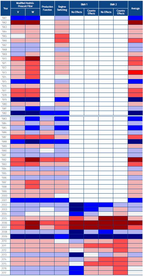
Note: Light to darker blue represents an observed growth slightly, one standard deviation, and two standard deviation below from its potential, respectively. Light to darker red represents an observed growth slightly, one standard deviation, and two standard deviation above from its potential, respectively. Light gray shows coincidence.
It is not possible to rule out a pre-pandemic new normal in CADR, this slowdown is evident since the 2008-2009 crisis, the outcomes from the statistical and structural approaches underscore two pre-pandemic stylized facts. On the one hand, the statistical methods show higher potential growth than structural models, indicating both a favorable context that CADR experienced and that the region would be closer to structural growth during a less favorable environment. On the other hand, most of the individual effects are negative: Therefore, in recent years these particularities seem to be making potential growth lower than it should be.
This approach accounts for particularities and allows concluding their presence; nevertheless, it does not identify specific determinants per country that might be causing dissimilarities in growth. Some researchers have attempted a growth diagnostic framework to identify binding constraints in the region, as shown below.
For Central American countries, Guasch, Rojas-Suárez, and Gonzales (2012) identify innovation, knowledge transfers, infrastructure or logistics, education or human capital, and crime or weak governance as critical areas to improve. Martin (2015) suggests that the high cost of capital, the anti-export bias,19 and the poor road and port infrastructure are limiting the growth of Belize. For Costa Rica, Beverinotti et al. (2014) find that infrastructure, scarcity of skilled labor in strategic areas, inadequate production linkages of small/medium companies with transnationals (free trade zones), and the fiscal deficit are constraining the economic growth. Also, Inchauste, Morena, and Stein (2009) and Asocio para el Crecimiento (APC, 2011) conclude that coordination problems between investment- promoting agencies, business training institutions, universities and the private sector, as well as crime and violence issues and low productivity in the tradable goods sector are restricting the growth in El Salvador. Sánchez, Scott, and López (2016) show how socioeconomic fragmentation, limited job opportunities, problematic human capital accumulation, limited capacity for provision of public goods, and occurrence of natural disasters are harming the growth of Guatemala (a performance widely shared with El Salvador, Honduras, and Nicaragua).
On the other hand, studies focused on productivity in the region (Schipke and Desruelle, 2007, and Sosa, Tsounta, and Kim, 2013) conclude that the productivity levels have not been sufficient to drive more growth.20 Table 7 summarizes some constraints of economic growth exposed in recent literature.
Table 7 Main Particularities Suggested by Authors
| Infrastructure | Human Capital | Crime and Violence | Exposure to Natural Disasters | Provision of Public Goods | Costs of Investment | Productivity | |
| Central America: Guasch, Rojas-Suárez, and Gonzales (2012) | X | X | X | ||||
| Belize: Martin (2015) | X | X | |||||
| Costa Rica: Beverinotti et al. (2014) | X | X | X | ||||
| El Salvador: Inchauste, Morena and Stein (2009), and APC (2011) | X | X | X | X | |||
| Guatemala: Sánchez, Scott and López (2016) | X | X | X |
Conclusion
Central America and the Dominican Republic have been experiencing a decline in potential growth. Statistical and structural approaches (Hodrick-Prescott filter by constrained minimization, production function, regime-switching models, and Bayesian model averaging) confirm the aggregate slowdown. This context could be understood as a pre-pandemic economic new normal in the region. Nevertheless, the findings suggest mixed results by country.
Most countries show a relative deacceleration of observed and potential growth and pre-pandemic macroeconomic conditions hindering their recent shock response. This situation constitutes another issue to highlight; the economic effects of the pandemic on the region could deepen the aggregate slowdown of the potential growth.
I identify at least two stylized facts: firstly, statistical models show higher potential growth signaling that in a less favorable context, the region would be closer to the structural growth; secondly, it is essential to consider particularities that might be structurally limiting potential growth. The approaches in this paper account for specificities and allow to conclude their presence, still, these methodologies do not identify specific determinants per country that might be constraining and causing dissimilarities in growth. This concern is an open gap that valuable further research should explore and fill in.

