English (pdf)
 Article in xml format
 Article references
 Send this article by e-mail
 Cited by SciELO
  Cited by Google
  Similars in
SciELO
Similars in
SciELO  Similars in Google
 Permalink
1. INTRODUCTION
In short, the Phillips curve is still there. But its current shape raises serious challenges for monetary policy in the future.
Oliver Blanchard, 2016
My view is that the data continue to show a relationship between the overall state of the labor market and the change in inflation over time. … I believe it continues to be meaningful for monetary policy.
Jerome H. Powell, 2018
Circuito Escolar s/n, Building B, Office 305, Postal Code: 04510, Mexico City, Mexico.
This article is part of the research project “Post-Covid society and economy in Mexico” (IN308021), DGAPA, UNAM.
A. W. Phillips (1958) found a negative and apparently stable relationship between the growth rate of monetary wages and the unemployment rate for the UK (1861- 1957). Later, Samuelson and Solow (1960) generalized this relationship by applying it to the United States (1934-1959) and called it Phillips Curve (PC). In their new version, inflation (the Consumer Price Index rate of growth) was explained by the unemployment rate and from then on was incorporated into the theoretical body of neoclassical synthesis as a central instrument of economic policy.
Since then, the form, strength, and theoretical and econometric characteristics of the PC have been central to the development of economic theory and it has become a fundamental tool for macroeconomic policymaking, particularly monetary.
With the incorporation of rational expectations (Muth, 1961; Lucas, 1972; Lucas and Raping, 1976), it was assumed that the PC would become vertical even in the short run if agents could anticipate or adapt quickly to the expansionary demand policy, thereby generating only inflation with an invariant unemployment rate.
However, by accepting that there are nominal rigidities that allow the existence of suboptimal equilibria in the short term, the New Keynesian Approach -represented by Blanchard (2008); Blanchard, Dell’Ariccia and Mauro (2010); and Carlin and Soskice (2015)- recovers the trade-off between inflation and the unemployment gap, albeit within a fully rehabilitated microfounded theoretical approach, and assumes that although the PC is vertical in the long run, in the short run there are real effects derived from shocks and economic policy.1
In this context, Galí and Gertler (1999) GG introduced a microfounded specification of the original PC that considers the nominal rigidities based on the idea of the phased price increase of Calvo (1983). Since then, the Hybrid New Keynesian Phillips Curve (HNKPC) considers expectations (both adaptive and rational)2 and the real marginal cost (as a measure of the business cycle) as crucial variables in determining inflation, which reflects the behavior of labor markets.
According to Ramos-Francia and Torres (2008) RFT, this specification has three advantages over the previous ones: 1) it allows modeling the pricing process within a monopolistic competition with firms that have temporary limitations to set prices; 2) it considers the formation of expectations as a prospective (rational) and a retrospective (adaptive) process; and 3) it uses a more adequate indicator of the business cycle, referred to marginal labor costs.
The PC is central to the macroeconomic theory and even more to economic policy, since it is probably the most important analytical, diagnostic, and action tool available for central banks to determine their monetary policy stance. In addition, according to Rumler and Valderrama (2010), this curve is the most efficient tool to make long-term inflation forecasts, which is what concerns the central banks the most. Nevertheless, although the estimates of this curve for the United States and Europe are abundant, in Mexico, despite its long history of inflation, there are very few applications and there are no official nor academic systematic estimates available; the most recent academic publication for Mexico is that of Cunha (2017). On the other hand, only Rodríguez (2012) incorporates the individual effect of the exchange rate in his estimate notwithstanding that according to RFT (p. 276), “given that Mexico is a small open economy, including variables that measure changes in relative prices with respect to the rest of the world (e.g., exchange rate variations) improves the results”.
We update the HNKPC inflationary dynamics analysis and we strengthen it by incorporating the real bilateral exchange rate (Mexico-United States) affecting the real marginal cost to analyze the impact of the external sector on the labor market, and subsequently on inflation through the labor market.3 Since all the variables are stationary, I(0), we use the Generalized Method of Moments (GMM) Hansen, 1982; and Hansen and Singleton, 1982 to estimate closed and open economy versions of the HNKPC for Mexico (2002Q1-2020Q1), thus obtaining asymptotically efficient and consistent non- autocorrelated nor heteroscedastic estimators and solving the possible endogeneity and simultaneity problems that could exist between the inflation expectation and the error term. We chose this period because it corresponds to the formal adoption of Inflation Targeting by Banco de Mexico (Ramos-Francia and Torres, 2005) around its long-term operational target, that since 2002 has been set at 3% ± 1%.4
We found the following to be the main results: a) there is robust empirical evidence that the HNKPC applies for the Mexican economy, so it offers a guide to understand the inflation dynamics and the monetary policy, and shows that inflationary expectations respond to both prospective and retrospective rules, while the business cycle measured with the real marginal cost -where the exchange rate is included-positively impacts inflation; b) by testing in-sample and pseudo out-of-sample forecasts accuracy (with expanding and rolling windows), for the open economy and closed economy versions, which is one of our main contributions, we prove that the open economy specification fits better the inflation data and provide better forecasts than the closed economy version of the curve; c) we find two structural changes (2009Q2 and 2017Q1) that can be associated with the Great Recession and with the onset of the latest inflation episode in Mexico; d) following the 2008-2009 financial crisis, this version of the PC has strengthened; f) the real marginal cost gap is more appropriate indicator of the business cycle than the output or unemployment gaps given that these variables produce inconsistent results with the economic theory;5 and g) in order to rule out the existence of nonlinearities in this version of the PC, we prove that there is no evidence of asymmetries or diminishing marginal returns coming from monetary policy.
The work is organized as follows: in addition to this introduction, in section two we conduct a literature review, in the third section we present the stylized facts of the main variables, in section four we present the econometric issues, in the following section we discuss the main statistical results, and finally, we conclude.
II. LITERATURE REVIEW
Applied studies of the HNKPC are abundant for the United States and Europe, and there are some studies for Latin America, but for Mexico there are very few, including those of RFT, Rodríguez (2012), and Cunha (2017).
According to Medel (2015), the main methodological differences that arise when estimating this version of the PC reside in the variables used to approximate inflation expectations and the business cycle. Stock and Watson (1999) point out that using the output gap offers better results if the objective is to make inflation forecasts. However, GG; Galí, Gertler and López-Salido (2005), and RFT emphasize the importance of using real marginal costs as a measure of the business cycle because the output gap is usually not significant, generates aberrant parameters or, as in our case, the estimation presents opposite sign. An additional advantage is that the marginal costs incorporate the possible effect of gains or losses in efficiency (labor productivity) on inflation.
Cermeño, Villagómez and Orellana (2012) explain that there are essentially two ways to incorporate rational inflation expectations: a) by taking proxy variables that could come from surveys, newspapers and forecast consensus, or b) like GG and RFT did it -and the way we make it in this work- assuming that expectations equal the first lead of inflation data (i.e. π E=π ). In this respect, Nunes (2010) estimates the HNKPC -in its reduced and structural versions- for the United States (1968Q4- 2007Q4) using inflation leads and information from surveys and forecast consensus as measures of the rational expectations. He finds that, although the latter is a good approximation for rational expectations, the former one has greater explanatory and predictive power of inflationary dynamics.
According to Ferreira et al. (2018), the HNKPC is fundamental for the decision-making of the central banks since they can implement disinflationary policies minimizing social costs,6 mostly if inflation is a prospective process. This explains the systematic effort of the central banks to anchor inflationary (forward) expectations and, thereby, avoid second-order effects.7 By doing so reduces the real effects generated by the policy. These authors find that, if inflation has a high retrospective component, indicating inflationary persistence, the sacrifice ratio of disinflationary policies is higher. In this way, the correct estimation gives the central bank the empirical elements to define the best (most efficient) stabilizing policy.
GG were the first in estimate the HNKPC for the United States (1960-1997) and found that expectation and the real marginal cost gap are significant to explain inflation. They show that the prospective component of inflation is much higher than the retrospective one.
Nason and Smith (2005) estimate the HNKPC for the United States (1949Q1-2002Q1), England (1961Q1-2000Q4), and Canada (1963Q1-2000Q4) and find in all cases a positive and significant relationship between the real marginal cost gap and inflation. They warn that the estimates are very sensitive to the Instrumental Variables (IV) and making estimates with different IV they find that in the United States rational expectations have always a greater impact than the adaptive ones.
For the Euro Zone (1970-1998), Galí, Gertler and López-Salido (2001) find that the prospective component is statistically significant, greater than the retrospective one and higher than that observed in the United States, and that the HNKPC fits better in the European Union than in the United States.
Vašíček (2011) estimates the open economy HNKPC (OEHNKPC) for four European Union economies (Czech Republic, Hungary, Poland and Slovakia) and finds, unlike us, that the real marginal cost might not be the best measure to approximate the business cycle, that inflation is determined in an important way by external factors, and that for these small economies the inflationary persistence is greater than in the developed ones.
For Hong Kong (1983-2002), Genberg and Pauwels (2003) estimate the OEHNKPC, and they find that the model fits better by incorporating the cost of imported inputs in the measure of the real marginal cost and the adaptive expectations component is higher than that of the rational one. They also warn about the sensitivity of the parameters to the set of IV.
Medel (2015) finds -with monthly data for Chile (2000-2013) - that the HNKPC has the capacity not only to explain inflationary dynamics, but also to make short-term forecasts. He estimates an unrestricted version of the HNKPC and shows that it is more efficient than the version that considers only the retrospective component and verifies the robustness of its results by estimating the same specifications for core inflation. He also estimates open economy versions8 and concludes that neither the real exchange rate nor the price of oil is statistically significant to inflation.
For Brazil (2001-2015), Ferreira et al. (2018) argue that the HNKPC generates different results depending on the variable used to measure the business cycle. They make several estimates using the three gaps (output, unemployment, and real marginal cost), in combination with two different measures of inflation expectations.9 They find that the output gap is either not statistically significant or shows the opposite sign to that predicted by the theory.10 In addition, under the hypothesis of lower foresight capability by firms, inflation is more sensitive to the cyclical component of economic activity. They find that inflation is more sensitive to its retrospective component, indicating greater inflationary persistence and the importance of high inflation history in the country.
Chowdhury and Sarkar (2017) use the output gap to estimate the BRIC economies PC (1994-2011). They find structural change and divide the estimates into two subperiods. By doing that, they show that both the prospective and retrospective components are significant, where the first one is in a range of 0.608-0.766, while the second one is between 0.218-0.387. The parameter of the output gap in most cases was not significant.
For Mexico we find only three references. RFT estimate the curve with monthly data (1996-2006) using the real marginal cost gap calculated as the logarithmic deviation of the unit labor cost of the manufacturing industry with respect to its trend, as it is done in the present work. They find that all parameters are statistically significant and that when the simple specification of the PC is used,11 the short-term dynamics of inflation is largely explained by its own lags; that is to say, inflation shows great persistence. However, when estimating the HNKPC they find that both types of expectations are statistically significant, as well as the real marginal cost gap. In addition, they show that inflationary persistence decreased at the end of the period; so, to a greater extent, inflation was explained by its prospective component.
The second reference for Mexico is that of Rodríguez (2012), who estimates the HNKPC for 1969-2008 with annual data using the output gap and incorporating the real exchange rate and the real wage as additional regressors. He finds that the closest lag of inflation is the most important in explaining it and that, although the prospective factor of inflation is significant, the estimates are not robust because it requires a very large number of IV to obtain satisfactory results and reducing them results in incorrect signs.
Finally, Cunha (2017), for 2001-2015,12 unlike GG and RFT, uses the output gap and his estimation method (Two-Stage Least Squares and State-Space) differs from that used by the bulk of the literature (GMM). In his estimate, there is evidence that both prospective and retrospective components are significant in explaining core inflation, in addition to being more important, in relative terms, than the output gap and imported inflation. Unlike RFT, he finds that the retrospective component gained strength against the prospective one.13
III. STYLIZED FACTS
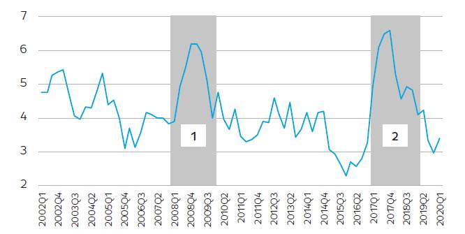
Figure 1 shows the evolution of inflation (π t ) in Mexico, defined as the annual growth rate of the National Consumer Price Index (NCPI) INEGI, 2020a.14 Since 2001 Banco de Mexico has formally adopted the inflation targeting approach (Ramos-Francia and Torres, 2005), which explains that since 2002Q1 inflation has reduced and has been essentially stable, so it presents a stationary behavior (Table IA of the Statistical Appendix) fluctuating at an arithmetic average of 4.25% and a standard deviation of 0.96. It is worth mentioning that just a few years before inflation used to be much higher, for example, in 1998 it reached 18% and in 2000, 11%.
Source: Prepared by the authors with data from INEGI (2020a).
Figure 1 Inflation (NCPI, annual growth rate), 2002Q1-2020Q1
During the analyzed period there were two inflationary episodes: 2008Q1-2009Q4 of essentially foreign origin (Great Recession), in which inflation reached up to 6.2%; and 2017Q1-2019Q1, whose origin was essentially domestic -although external factors were also involved-, during which it reached up to 6.6%. The former is explained by increases in the international prices of raw materials and by strong exchange depreciations that began in September 2008 as a result of the Great Recession (Banco de México, 2009). The latter was explained by the increase in the prices of food and non-food goods, agricultural and energy products,15 the increase in the minimum wage (December 2017) and the exchange depreciation explained by the fear of the electoral triumph of Donald Trump in 2016 (“Trump Effect”) Martínez, 2017; Díaz, 2018; Expansion, 2019. If we eliminate these two episodes, the mean and standard deviation for the entire period is 3.96 and 0.64, respectively.
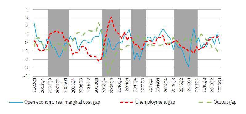
Figure 2 shows the gap for the open economy real marginal cost (mc OE). Negative gaps are mainly associated to: a) imported recessions (dot com crisis in 200116 and the Great Recession in 2009) which caused strong declines in employment and in the real wage in manufacturing, and important exchange rate depreciations in Mexico (see Figure 3); and b) strong reduction in the wage bill combined with the increase in average labor productivity (2011-2012 and 2015-2016) Banco de México, 2012 and with a strong exchange depreciation in 2016 (see Figure 3), respectively. This clearly shows that, consistent with our theoretical approach, recessions and depreciations17 reduce -with lags- the real marginal cost (below their steady state trajectory) due to the loss of workers’ negotiation power.
Source: Own estimate with data from Banco de México (2020), Federal Reserve Bank of St. Louis (2020) and INEGI (2008, 2020a and 2020b).
Figure 2 Gaps: open economy real marginal cost, unemployment, and output Normalized data, 2002Q1-2020Q1
Note: gaps are calculated with the Hodrick Prescott filter Hodrick and Prescott, 1997. To be visually comparable, data were normalized by the following statistical procedure: where the arithmetic mean and σ is the standard deviation.
It is easy to see that the real marginal cost gap is less volatile than the output and unemployment gaps, which highlights the nominal rigidities that lower the sensitivity of the relation between the real average pay and average productivity, given the dynamics of the business cycle.
Figure 3 contrasts the open economy real marginal cost gap (mc OE) with that of closed economy (mc CE). Calculation process can be found in equations (1B) and (2B) in the Methodological. It is noteworthy that, although they present essentially the same evolution, the measurement of the closed economy is smoother, indicating that the exchange rate increases the business cycle volatility.
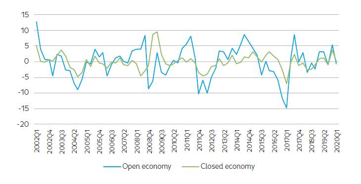
Note: Data is presented as logarithmic deviations, so they reflect the quarterly percentage deviation with respect to their stationary state value. Source: Own elaboration with Banco de México (2020) and INEGI (2008 and 2020b) data.
Figure 3 Open and closed real marginal cost gaps, 2002Q1-2020Q1
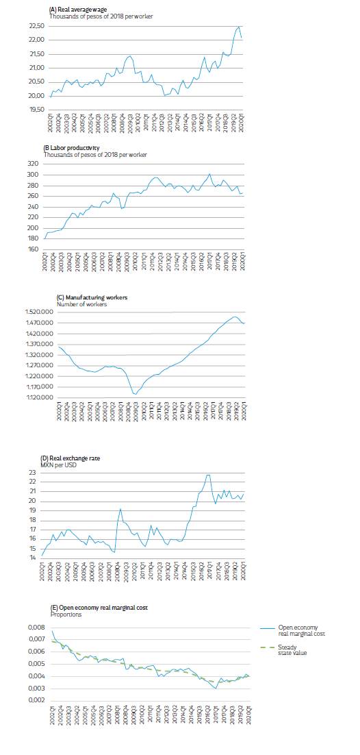
Figure 4 shows the unit marginal cost and its steady state value (panel E), and the four factors that make up this measure of the business cycle (panels A, B, C and D).
IV. ECONOMETRIC ISSUES
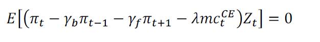
In this paper, we estimate the HNKPC for open economy (OEHNKPC, equation 1) and for closed economy (CEHNKPC, equation 2):
 (1)
(1)
 (2)
(2)
Where mc t OE and mc t CE are the real marginal cost gaps for open and closed economy, respectively, and are calculated as the logarithmic percentage deviations of the marginal cost for open economy (MC t O) and closed economy (MC t CE), in each case, related to their steady state values obtained with the Hodrick Prescott filter (Hodrick and Prescott, 1997). π t-1 and π t+1 are the retrospective and prospective components, respectively.
Like RFT, we implicitly assume a Cobb-Douglas production function, so the marginal cost equals the Unit Labor Cost, whose specification for closed and open economy can be found in equations (1B) and (2B) in the Methodological.
The estimates of (1) and (2) are for 2002Q1-2020Q1 due to the formal adoption of the inflation- targeting approach and that inflation became stationary since 2002Q1, which is required by GMM approach. In Table IA we prove that all variables are integrated of order 0, I(0).18
According to Cermeño et al. (2012), incorporating the expected values of a variable -such as the rational expectation of inflation Eπ t+1 - can be done by assuming that ex post values are equal to their expected values plus a forecast error term (π t+1 = E π t+1 +ε t+1 ), so that these values can be used to model inflationary expectations of the form E π t+1 = π t+1 -ε t+1 , which can generate endogeneity and simultaneity in the estimate because can be correlated with the residual ε t+1 .
To avoid this problem, the literature on the subject suggests using GMM (Hansen, 1982; Hansen and Singleton, 1982) which consists in the selection of a set of instruments that should be correlated with the regressors but not with the residual term, accomplishing the orthogonality condition for the two specifications:
 (3)
(3)
 (4)
(4) The high sensitivity of GMM estimates due to IV has been widely documented (Nason and Smith, 2005), so to address this problem, we selected the most efficient IV set by making a wide number of estimations with different sets that accomplished statistical significance, goodness-of-fit, Schwartz and Hannan-Quinn criteria (Andrews, 1999), and the Criterion on Relevant Moment Selection (Hall, Inoue, Jana and Shin, 2007).19
Outputs are presented in Table I, where it is observed that in both estimates all the parameters are statistically different from zero and, according to the J-statistic, it cannot be rejected that equations are correctly overidentified.
Table I Estimates of the open and closed economy HNKPC, 2002Q1-2020Q1
| Parameter | Open economy 3/ | Closed economy 4/ |
| γb 1/ | 0.471 (9.850) | 0.153 (1.962) |
| γf 1/ | 0.531 (10.661) | 0.852 (10.510) |
| λ 1/ | 0.025 (2.752) | 0.046 (3.996) |
| R2 | 0.803 | 0.725 |
| J-Stat 2/ | 4.125 (0.531) | 4.810 (0.307) |
1/ In parenthesis t statistic.
2/ P-value in parenthesis.
3/ Instruments: π t 2 and 3 lags, output gap (Y G) 2 to 5 lags, unemployment gap (U G) 2 to 5 lags, US annual GDP growth rate (Y US)
5th lag and the first difference of the bilateral real exchange rate (Mexico-US) ∆q t current, 1 and 2 lags.
Y G and U G were calculated with the HP filter.
4/ Instruments: π t current, 1 and 2 lags, mc CE current and 1 to 5 lags, ∆q and the first difference in the real interest rate (∆r ) 4th lag.
r t =i t -π t where r t is the real interest rate, and i t is the nominal interest rate (28 days-CETES).
All IV were obtained from Banco de México (2020), Federal Reserve of St. Louis (2020) and INEGI (2020a). The HAC weighting matrix was used in all estimates to obtain consistent and efficient estimators.
Table IIA shows that instrumental variables are orthogonal to the error.
It should be noted that the model was estimated until 2020Q1 because when incorporating the following quarters, despite the parameters associated with the prospective and retrospective components remain almost unchanged, the ones associated with the marginal cost gap alters significantly. This result shows that as usual, inflation is especially sensitive to the slack in the business cycle.
V. DISCUSSION
To evaluate the explicative capacity of (1) and (2) we tested in-sample-forecast and pseudo-out-of-sample forecast for 2017Q1-2020Q1.20
We observe that the open economy specification generates a more accurate forecast since the performance statistics are lower due to the distance between the forecasted and observed errors are minimized, see Table II.
Table II Forecasts accuracy: fixed window
| Accuracy statistic | Open economy | Closed economy |
| In-sample forecast | ||
| RMSE | 0.419 | 0.496 |
| Theil | 0.048 | 0.057 |
| MAE | 0.347 | 0.406 |
| Pseudo out-of-sample forecast | ||
| RMSE | 0.461 | 0.521 |
| Theil | 0.047 | 0.053 |
| MAE | 0.426 | 0.428 |
Complementarily, we use the expanding and rolling window schemes to evaluate the estimations forecast accuracy at different horizons.
In both cases, the first window started in 2002Q1 and the last one in 2018Q4. We set the forecast to 4 quarters onward. In the second procedure, the window rotated 8 times and we considered 50 quarters.21
Table III shows that with both approaches the specification for the open economy generates more accurate inflation forecast for all horizons.
Table III Pseudo out-of-sample-forecasts accuracy: expanding and rolling window
| Open economy | Closed economy | |||||||
| h quarters ahead | 1 | 2 | 3 | 4 | 1 | 2 | 3 | 4 |
| Expanding window | ||||||||
| Bias | 0.279 | 0.284 | 0.259 | 0.166 | 0.385 | 0.554 | 0.742 | 0.477 |
| RMSE | 0.628 | 0.708 | 0.622 | 0.567 | 0.795 | 0.836 | 0.891 | 0.670 |
| MAE | 0.565 | 0.598 | 0.462 | 0.414 | 0.613 | 0.673 | 0.742 | 0.560 |
| Rolling window | ||||||||
| Bias | 0.314 | 0.327 | 0.287 | 0.182 | 0.421 | 0.609 | 0.802 | 0.512 |
| RMSE | 0.681 | 0.785 | 0.657 | 0.583 | 0.820 | 0.895 | 0.937 | 0.690 |
| MAE | 0.590 | 0.645 | 0.478 | 0.404 | 0.629 | 0.713 | 0.802 | 0.569 |
Thus, RMSE and MAE, after considering the variance and the forecasting bias, confirm that by incorporating the exchange rate the forecasting accuracy improved the dynamics of Mexico’s inflation. Subsequently, the rest of the analysis is completed on that specification.
The statistical significance of the estimated parameters demonstrates that OEHNKPC fits the inflation process in Mexican economy and the values of γf and γb claim that economic agents form their expectations according to prospective and retrospective rules: 0.53 vs. 0.47, respectively. The λ parameter indicates that for each percentage point that mc OE is above its long-term value, inflation increases by 0.025. Table IV shows that output and unemployment gaps have an inconsistent relationship (statistically significant but with opposite signs) to inflation, as pointed out by GG and Ferreira et al. (2018), proving that using the real marginal cost gap as an indicator of the business cycle -as it is done in this paper- is appropriate
Table IV Estimates of the closed economy HNKPC with different measures of business cycle, 2002Q1-2020Q1
| Parameter | Y t G 1/ | U t G 2/ |
| γb | 0.304 (9.014) | 0.370 (13.629) |
| γf | 0.697 (18.834) | 0.632(24.041) |
| λ | -0.067 (-2.999) | 0.206 (2.545) |
| R2 | 0.785 | 0.807 |
| J-Stat3/ | 7.48 (0.06) | 1.97 (0.853) |
t-statistic in parenthesis.
1/ Instruments: π t 1 to 3 lags, Y G 1 to 5 lags, U G 1 to 3 lags, π .
2/ Instruments: π t , π t 1 to 2 lags, U G 1 to 3 lags, Y G 1 to 3 lags, mc OE 1 to 4 lags and ∆r t 1 to 6 lags.
3/ P-value in parenthesis.
Another main issue in the literature is about the presence of non-linearities. Accordingly, we estimate the quadratic functional form that turned out to be statistically non-significant in both parameters of marginal costs. Thus, we rule out the fact that the OEHNKPC estimated here presents asymmetries and diminishing marginal yields of the policy, Table V.
Table V OEHNKPC quadratic functional form, 2002Q1-2020Q1
| Variable | Parameter |
| π t-1 | 0.421 (7.238) |
| π t+1 | 0.594 (9.455) |
| mc t OE | 0.016 (1.215) |
| mc t OE 2 | -0.002 (-1.287) |
| R2 | 0.805 |
| J-Stat3/ | 4.475 (0.483) |
t-statistic in parenthesis.
Instruments: π t 2 and 3 lags, Y G 2 to 5 lags, U G 2 to 5 lags, Y US 5th lag ∆q current, 1 and 2 lags.
3/ P-value in parenthesis.
Regarding the results for developed countries (GG and Galí et al., 2001) and in this work (for the entire period), the prospective component is higher than the retrospective one; while in developing economies such as Brazil (Ferreira et al., 2018), with strong inflationary history, the retrospective component is higher.
For Mexico, RFT (1992M1-2006M6) -for closed economy- find that both components are similar, but that the prospective one has gained strength since 1997, which points out in the same direction as the one we found here. Rodríguez (2012) estimates for the open economy and obtains results that show that the prospective component is higher, but there are inconsistencies with his estimate due to the expectations parameters sum is very different from one. Finally, Cunha (2017), who also estimates for the open economy, claims that the rational expectations component is higher.
We found that our business cycle parameter is similar to that for developed economies (GG and Galí, et al., 2001), but is very low compared to that for developing economies (Medel, 2015; Ferreira et al.,2018).22 We also found that this relationship has strengthened given that it is higher than the estimated by RFT and more similar to that of Cunha (2017).
By applying the Andrews-Fair Wald and Andrews-Fair LR-Type D tests (Andrews and Fair, 1988) we found two structural changes in the regression in 2009Q2 and in 2017Q1, see table IIIA. Both dates coincide with the beginnings of inflationary shocks. From the first structural break we suggest that the Great Recession had permanent strong recessive and inflationary effects in Mexico, and it is likely that it modified the inflation dynamics in terms of its relation between the labor market and pricing, and even in the formation of agents’ expectations. To prove it, we estimated by subperiods, see Table VI.23
Table VI OEHNKPC. Estimates by sub-periods
| 2002Q1-2020Q1 | 2002Q1-2009Q1 | 2009Q2-2020Q1 | |
| γb | 0.471 (9.85) | 0.42 (10.51) | 0.458 (8.79) |
| γf | 0.531 (10.66) | 0.58 (14.74) | 0.544 (9.53) |
| λ | 0.025 (2.75) | -0.01 (-1.50) | 0.026 (2.54) |
| R2 | 0.80 | 0.81 | 0.81 |
| J-Stat1/ | 4.125 (0.531) | 3.37 (0.643) | 4.39 (0.49) |
t statistic in parenthesis.
1/ Ho: the instruments are jointly valid. P-value in parenthesis.
Instruments: π t 2 and 3 lags, output gap (Y G) 2 to 5 lags, unemployment gap (U G) 2 to 5 lags, US annual GDP growth rate (Y US) 5th lag and the first difference of the bilateral real exchange rate (Mexico-US) ∆q t current, 1 and 2 lags.
HAC weighting matrix was used in order to obtain consistent and efficient estimators.
For the entire sample and for the two subsamples both components -prospective and retrospective- are quite similar. However, for the period 2002Q1-2009Q1, the business cycle is not statistically significant, but rather it is statistically significant after the Great Recession.24 The results imply that since then the PC has strengthened given that the business cycle has greater impact on price setting, contrary to what occurred in other developed and emerging countries, where this impact decreased giving rise to the hypothesis of the flattening of this curve that has emerged in recent years.25
Finally, it would be interesting to analyze how inflation dynamics switched after the last structural change (2017Q1), which is associated to the onset of the most recent inflationary episode. Nonetheless, the lack of degrees of freedom does not allow to carry out this estimation. However, the presence of structural change allows to suggest that during inflation shocks, agents expectations and the sensitivity of inflation to business cycle could change.
VI. CONCLUSIONS
In order to update and strengthen the analysis of the inflation dynamics in Mexico, we estimate the OEHNKPC for the Mexican economy (2002Q1-2020Q1) with GMM by which we obtained asymptotically efficient, non-autocorrelated nor heteroscedastic estimators.
We demonstrate that this model keeps on fitting the determinants of pricing in Mexico since gives good explanation of the inflation expectations (both prospective and retrospective). Likewise, this approach explains that the business cycle measured through the real marginal cost gap has a significant and positive impact on inflation.
We also show that the open economy specification fits better the inflationary process and generates a more accurate and efficient in-sample and pseudo-out-of-sample-forecast, making it more suitable for economic policy.
We find that the open economy model reports structural change in 2009Q2 and in 2017Q1, which coincides with the beginning of the Great Recession and the impact of inflationary domestic policies, respectively. Although after 2009Q2 the formation of expectations was not modified, the impact of the business cycle on inflation was notably greater, suggesting that the PC in Mexico is not flattening as it occurs in other economies, developed and developing. On the other hand, it is plausible to suggest that after 2017Q1 the inflation dynamics could have affected the formation of expectations and the sensitivity of inflation to the business cycle. However, the absence of degrees of freedom prevents us from proving it econometrically.
In addition, and in line with GG and Ferreira et al. (2018), we find that both the unemployment gap and the output gap give opposite sign to that claimed by the theory, whereas using the marginal cost gap, satisfactory results are obtained. Similarly, there is no evidence of non-linearities within the model, which indicates the absence of asymmetries in inflation determination under this approach and that monetary policy has no diminishing marginal yields.