


 Inglês (pdf)
 Artigo em XML
 Referências do artigo
 Enviar este artigo por email
 Citado por SciELO
  Citado por Google
  Similares em
SciELO
Similares em
SciELO  Similares em Google
 Permalink
1. Introduction
The World Health Organization declared the novel COVID-19 outbreak a public health emergency of international concern on January 30, 2020. By the end of that year, on November 9, Pfizer and BioNTech announced their coronavirus vaccine had an efficacy rate of over 90%, and in December, the U.S. Food and Drug Administration granted them the first emergency use authorization. The space between those two events was a unique period in time when humanity as a whole faced a difficult situation whose outcome was unknown, that of the global spreading of a deadly infectious disease with no vaccines at hand. However, the COVID-19 pandemic was more than a global epidemic that disrupted international mobility, transport and trade in that period. It became a complex dynamic mix of COVID-19's epidemiology, government's health, economic and social policy, and community, household and individual reactions and decisions particular to each country. These constitute what is referred to here as the pandemic shock, which impacted all countries under highly heterogeneous initial conditions. Beyond the wide variation of COVID-19 cases among countries, the pandemic shock also had an inevitable secondary effect, the reduction of the economic activity in the countries, which is the topic of interest in this article.
The follow-up of the pandemic's shock economic effects was generally observed through the quarterly variation of standard macroeconomic performance measures or outcome variables and their short-term forecast, produced by country governments and international organizations like the IMF's World Economic Outlook (2021). A more challenging task was attempting to explain the behavior of those economic outcome variables based on the source of pandemic shock variables and their interactions (Pragyan et al., 2020; Furceri et al, 2021; Bakker & Goncalvez, 2021). Understanding and measuring the pandemic's economic impact is essential for several reasons: (i) governments need to understand the transmission channels to economic recession and its characteristics in order to adjust the health, economic and social policies; (ii) they need to follow up the economic recovery, its characteristics, pace and recoils; (iii) they need to understand the changes in household's decisions concerning labor, health and safety risks given the wide range of circumstances.
In a pre-vaccines COVID-19 world, infections, the policy effectiveness, the international context and the initial conditions will impact the country's population who, down to the household level, would generate an outcome expressed in social distancing behavior and some proportion of COVID-19 cases. The outcome would provide feedback on complementary policies under changing degrees of strictness and COVID-19 dynamics. The outcome of confronting COVID-19 in the health domain produces a predictable but inevitable secondary impact on the economic domain. It reduces the population's demand and the companies' supply of goods and services, affects their supply chains and produces unemployment and capital loss, thus affecting the national economic activity. Some authors interpret this as a trade-off between actions and outcomes in the health domain with actions and outcomes in the economic domain (Carrieri et al., 2020; Hall et al, 2020; Ceylan et al., 2020; Famiglietti & Leibovici, 2021; Bargain and Aminjonov, 2020; Fukao & Shioji, 2021). Governments have designed complementary policies to lessen the impact on the economy of households, companies, the government itself, and employment. However, the problem of loss of aggregate economic activity can only be solved in the health domain when COVID-19 is eventually defeated or at least contained. This solution was not available in 2020.
The vital aspect to notice in this complex interaction is that, in the end, it is the population who experiences the health and economic consequences of the pandemic shock and the one that connects the health domain with the economic domain. Their health outcome feeds back into COVID-19 policies and secondary economic policies. This perspective is the basis for the assumption in this paper that the people's observed behavior during the COVID-19 pandemic captures their health protection, risk decisions, and economic sacrifice decisions. A derived argument is that the COVID-19 policies and the COVID-19 do not directly affect the economic outcome but only indirectly through people's behavioral patterns regarding health risks and economic sacrifice within each household's economic circumstances. This line of argument justifies looking at people's behavior during the pandemic, and not just any behavior, but rather those most closely related to the central COVID-19 social distancing policy. This is why it makes sense to use country mobility data like Google's mobility trends, as this information could capture the complex interactions explained above and thus help explain the aggregate economic activity outcomes of 2020 (Sampi & Jooste, 2020).
This article concentrates on a specific relationship, that of people's behavior during COVID-19's first wave and its effect on the aggregate economy during 2020, mainly because this was a discovery period for humanity as a whole when the unknowns were dominant and a source of genuine fear while the possibility of a vaccine was only a desirable idea. Today we have access to information about people's behavioral patterns during COVID-19's first wave, which were recorded by Google (link provided in the references) and produced several mobility measures that can be used as explanatory variables in models that can help understand how recession happened on those early days. Models are estimated for one specific country, Bolivia, to test the strength of the correlation between the mobility measures, the trends and the general economic activity index (IGAE) as the outcome variable, which has its own structural and built-in forces for reproducing economic activity. The econometric strategy is to estimate individual ARMAX models relating the IGAE's growth rate to the growth rate of each type of mobility measure and to the growth rate of an aggregate mobility index. Models include seasonal dummy variables and autocorrelation components to capture the strength of structural characteristics and built-in forces of the Bolivian economy. All models were estimated assuming that the COVID- 19's first wave dynamics and government policies are not direct explanatory variables of aggregate economic activity but only indirect through people's mobility behavioral patterns. All models use the monthly IGAE time series from January 2015 to November 2020 published by the Bolivian National Institute of Statistics. The mobility measures are included as an explanatory variable only for the period of the COVID-19's first wave, from February to November 2020. The mobility data is published by OurWorldInData.org based on Google's COVID-19 Community Mobility Reports.
Bolivia was selected as a case study for several reasons. Firts, it is a Latin American developing country (US$3500 per capita GDP) where the degree of urbanization was already above 70% before the pandemic shock. Second, it has an Internet penetration of just above 50%, primarily through smartphones, significant governance limitations, and above 75% of economic informality. This last feature would be expected to make it particularly difficult for people to find a long-term balance between health protection and economic sacrifice, and the reason why household and individual learning and risk-taking were probably crucial for explaining the frequent changing of that balance as the Google data suggests.
The main finding is that the growth rate of the Bolivian aggregate mobility index is, in fact, positively correlated with the growth rate of the Bolivian IGAE index during COVID-19's first wave. The individual mobility measures of grocery & pharmacy visits and workplace visits are the most reliable to explain the influence of mobility on economic activity. The econometric results also show that the economic structure and built-in forces of the economy are a significant part of the explanation, but always together with the contribution of a mobility pattern.
Besides this introduction, Section 2 presents essential background information on the Bolivian COVID-19 experience, Section 3 explains the methodology and data, and Section 4 presents all the model estimation results and interpretations. Finally, the last section summarizes and suggests complementary research.
2. Antecedents
The design, implementation and effectiveness of policies were certainly crucial in confronting the pandemic caused by the COVID-19, and more so in its early days. Figure 1 conveys some basic information about COVID-19 policies during the ten-month period from February to November 2020, including a contrast between the daily Bolivian stringency index as recorded by Oxford (link provided in the references) and the daily Bolivian mobility measures as recorded by Google (link provided in the references). In the face of COVID-19 news arriving during February and early March, mainly from Europe, the Bolivian government decided to confront the inevitable impact with the closure of borders and a strict quarantine implemented from the third week of March to the first week of May. The next period of a flexible quarantine (under confinement recommendation) went from the second week of May to the end of August, and it essentially allowed for the household's own decisions regarding staying at home or going out with protection. The post confinement period began in September under restored mobilization and softer measures. Beyond these policies, the ECLAC's COVID-19 Observatory1 (link provided in the references) recorded 81 other policy actions taken by the Bolivian government during the first wave in the areas of health, movements across & within borders, economy, labor, social protection, education & schools, and gender. Other descriptions of the Bolivian COVID-19 policies can be found in Castilleja-Vargas (2020).
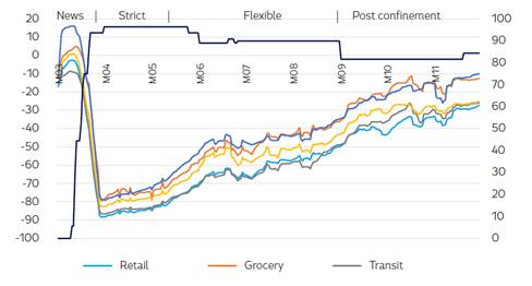
Daily variation of the stringency index is measured on the right axis. Source: OurWorldInData.org and Oxford’s Government Response Tracker.
Figure 1: Mobility patterns in relation to the policy stringency index
Figure 1 suggests that policy stringency remained high during the whole year, although it decreased over time (100 = strictest): highest during the strict quarantine (96,3%), decreasing from the end of May to the end of August during the flexible quarantine (89,8%), and decreasing again in the post confinement period (81,5%). However, stringency seemed to have differed significantly compared to people's mobility behavior2. The policies might have had a stronger influence on people's behavior and compliance during the strict quarantine period but much less so afterwards. In fact, the flexible quarantine resulted from compliance difficulties given the impossibility of extending the strict quarantine in the Bolivian economic and social context. It required critical economic sacrifices that most of the population could not afford. The figure shows that, in general, the mobility index caught an increasing tendency very early in April until November, changing only its slope steepness over time.
Figure 2 contrasts the daily variation of COVID-19 cases against the daily mobility measures and patterns over time. The mismatch between the period of the full COVID-19 wave and the strict quarantine period in the figure suggests that the latter might have been implemented either too early, for as much as two months, or had the effect of postponing the wave for the same amount of time. The fact is that from April to June, mobility was increasing together with the early part of the wave, and the flexible quarantine period might have let the wave follow its course instead of flattening it. When the wave peaked under an uncontrollable rise in COVID-19 infections from mid-July to mid August, apparently, it affected people's mobility by deterring it or at least slowing it down. This was part of a process where people were learning to live with the restrictions and assess risks, which was constantly changing the balance between staying home or going out. Later in the post confinement period beginning in September, together with the end of the COVID-19 wave, the relationship changes again as mobility takes an upward slope shift, with people massively increasing their mobility during a period of decreasing rates of COVID-19 infections. This is certainly a three-stage complex relationship, besides the known COVID-19 data generation problems (Glaubitz & Feng, 2020).
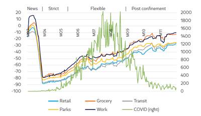
The daily variation of COVID-19 cases is measured on the right axis. Source: OurWorldInData.org
Figure 2 Mobility patterns in relation to COVID-19's first wave
In a closer look at the mobility measures and their trends, they began with an anticipation behavior in late February and early March. However, mobility really dropped in the second half of March, which is consistent with the government's emergency declaration and soon after the strict quarantine mandate during the third week of March. The mobility measures reached their minimum daily levels of -79% to -88% from March 29 to April 1, expressing a combination of COVID-19 fear and policy stringency. Kennedy et al. (2021) identify exemplar countries at epidemic preparedness and response in a prevention strategy (social distancing with lockdown as an extreme measure), detection (testing), containment (infection rates) and treatment (fatality rate) which was out of Bolivia's organizational reach in 2020. The mobility trends began to shift back upwards with a lower slope until the first week of May, but still with mobility levels lower than -70% and consistent with the end of the strict quarantine on May 10. The daily mobility patterns continued moving upwards with a steeper slope once the flexible quarantine mandate began on May 10, including the somewhat flattening in daily mobility from mid-June to mid-August (average daily mobility in the range from -46% to - 60%) when the COVID-19 wave reached its peak, and then increasing their slope back up again from mid-August (the flexible quarantine ended on August 30) to the end of the first wave on November 30 (average daily mobility in the range from -10% to -25%).
Figure 3 contrasts the behavior of the Bolivian monthly IGAE index as recorded by the National Institute of Statistics (INE) against the diverse measures of monthly mobility trends3. The impact of the pandemic shock on the Bolivian economy was measured by Barja (2021) as the accumulated difference between the observed IGAE time series and its counterfactual or how the economy would have behaved in the absence of COVID-19. Its computation produced an accumulated -12.6% loss of aggregate economic activity from February to November 2020.
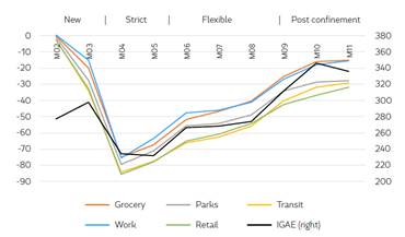
The monthly economic activity IGAE index is measured on the right axis. Source: OurWorldInData.org and INE.
Figure 3: Mobility patterns in relation to the IGAE index
The figure also provides information about the impact of COVID-19 policies on both variables, suggesting the strict quarantine had a strong secondary effect on the IGAE index, through the significant drop in the mobility measures in March and April, but not so much in May when mobility began increasing faster than the IGAE. However, the IGAE index seemed to have increased faster than mobility in June. Later, when the COVID-19 wave reached its highest level during July and August, which slowed the mobility recovery, this event, together with the COVID-19 itself, had the secondary effect of flattening the IGAE recovery even under a flexible quarantine policy. Afterward, when the COVID-19 wave began to recede and, consequently, mobility resumed its growth faster, it also had the positive secondary effect of increasing the IGAE's recovery to its highest level in October and November4. The hypothesis is that while Figures 1 and 2 tend to show the direct effect of the COVID-19 policies and the COVID-19 epidemiology on mobility, given the international COVID-19 context, Figure 3 tends to show their indirect effect on economic activity through the transmission channel of people's mobility behavior.
Besides the three complementary descriptions of the events presented above, there is a fourth element at stake related to the built-in forces within the Bolivian economic structure and the sectors that compose it, captured by the seasonal and autocorrelation patterns contained in the IGAE index, which might have been pushing for an increase in economic activity whenever it was possible. A large proportion of the Bolivian economy is an informal and extreme subsistence-type of economic activity which requires face-to-face transactions. Therefore, it is reasonable that the economic survival was valued over COVID-19's related health risks, after a learning period, even in the middle of a rising COVID-19 wave, while the smaller proportion of other types of companies was still able to contribute to the economy by working from home.
3. Methodology and data
The estimation strategy uses ARMAX-type models to establish an explanatory relationship from the time series of people's mobility to the time series of the general economic activity index (IGAE) during COVID-19's first wave, from February to November 2020. ARMA models were popularized by Box & Jenkins (1970) and Box, Jenkins & Reinsel (1994) for time series analysis and forecasting. A key advantage of the ARMA-type models is their ability to capture the natural regularities in time series through the autocorrelation and moving average contained in them. Another advantage is the possibility to include deterministic-type variables like seasonal dummies that can also help capture natural regularities contained in the data or some cases, explain extreme observations, and tendency type variables that can help capture natural linear or quadratic trends in the data. Moreover, the ARMAX models are a natural extension by including other exogenous explanatory variables (Davidson & MacKinnon, 2004, p. 565-566). The following is a representation of the basic ARMAX (p, q) model:
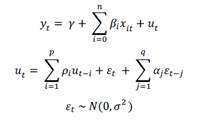
The first equation is a multiple regression of a stationary time series y t against explanatory stationary time series variables x. t , and y is a constant term but can also include deterministic seasonal dummy variables. The coefficients ¡3. measure the contemporaneous impact of the exogenous variables x. t . The second equation is an ARMA model of the residuals from the first equation, or stationary time series u t , against a linear combination of its own past p periods plus a linear combination of the innovation term q periods past; £ t is the innovation term or regression residuals. The ARMA process provides a way to model the evolution of the conditional mean of u t . The model assumes the regression residuals e t are normally distributed with zero mean and constant variance o 2 . The combined equations of the ARMAX (p, q) are estimated simultaneously by maximum likelihood methods. The econometric strategy in the context of the IGAE and the Mobility time series is to estimate ARMAX models for the stationary transformation individually in search of parsimonious models with the highest R-square and normally distributed white noise residuals in their mean and variance.
Regarding data sources, the IGAE time series can be freely downloaded from INE's website (link provided in the references), which also contains its methodology and sources of information. The mobility time series can be freely downloaded from OurWorldInData.org (link provided in the references). Annex contains the variable's order of integration, and annex their descriptive statistics.
4. The effect of mobility on economic activity during COVID-19's first wave
Table 1 presents the estimated models with particular characteristics. Model 0 explains the IGAE's growth rate without any exogenous explanatory variable. It was estimated for the pre-COVID-19 period from 2015M1 to 2019M10 and also previous to the November political conflict that the country experienced. The series begins in 2015 because it represents the first year after the end of the Bolivian economic boom that resulted from unusual high international prices of minerals and natural gas exports (the Bolivian growth model is based on commodity exports in exchange for industrialized imports). Its estimation shows that the IGAE's growth rate can be strictly modelled based on all its past observations. The economy's structural characteristics are captured by the monthly dummy variables, which are all significant, showing that the IGAE growth rate strongly follows a particular monthly pattern. A first-order moving average variable captures the internal dynamics or built-in economic forces. Model 0 basically summarizes the Bolivian economy from the perspective of its monthly patterns and dynamics in a straightforward format for reference purposes.
Table 1 Estimated models for IGAE's growth rate d(log(igae))
| Variables | Model 0 | Model 1 | Model 2 | Model 3 | Model 4 | Model 5 | Model 6 | Model 7 |
| d(mobility) | 0.005232** | |||||||
| d(grocery) | 0.005182** | |||||||
| d(retail) | 0.005049** | |||||||
| d(transit) | 0.004964** | |||||||
| d(work) | 0.005468** | |||||||
| d(parks) | 0.005342** | |||||||
| d(residential) | -0.011482** | |||||||
| d1 | -0.125111** | -0.113241** | -0.118939** | -0.090575** | -0.143818** | -0.113551** | -0.145295** | -0.115265** |
| d2 | -0.058200** | -0.071674** | -0.066587** | -0.073971** | -0.071272** | -0.072509** | -0.0799 06** | -0.063068** |
| d3 | 0.123540** | 0.138163** | 0.133600** | 0.122875** | 0.168051** | 0.131531** | 0.118510** | 0.137886** |
| d4 | 0.053230** | 0.058282** | 0.053121** | 0.077020** | 0.023677* | 0.064325** | 0.024480* | 0.052930** |
| d5 | -0.017492** | -0.033678** | -0.028802** | -0.034176** | -0.032930** | -0.035485** | -0.040406** | -0.028842** |
| d6 | 0.008984** | 0.021323* | 0.022436** | 0.050692** | 0.018708* | 0.023561** | ||
| d7 | -0.032978** | -0.021129* | -0.025541** | -0.052650** | -0.020220* | -0.057848** | -0.026370** | |
| d8 | 0.019506** | |||||||
| d9 | 0.062882** | 0.066445** | 0.066133** | 0.047328** | 0.094660** | 0.066795** | 0.044611** | 0.065441** |
| d10 | 0.024852** | 0.037374* | 0.035656* | 0.059854** | 0.034559* | 0.034009** | ||
| d11 | -0.044864** | -0.057700** | -0.055105** | -0.060611** | -0.054803** | -0.059595** | -0.061779** | -0.056844** |
| d12 | 0.023750** | 0.035034** | 0.031897** | 0.016963* | 0.060934** | 0.034110** | 0.013319° | 0.031343** |
| pcrisis | -0.031987** | -0.020690** | -0.039442** | -0.035784* | -0.015916* | -0.039510** | -0.034224* | |
| MA(1) | -0.612045** | -0.538106** | -0.502922** | -0.622895** | -0.590416** | -0.422646* | ||
| MA(2) | 0.507169* | |||||||
| MA(3) | 0.309282* | |||||||
| AR(1) | -0.573652** | -0.380291** | ||||||
| AR(2) | -0.631454** | -0.738708** | ||||||
| AR(3) | 0.603802** | 0.776237** | 0.766723** | 0.478106** | 0.660574** | |||
| AR(4) | 0.325940** | |||||||
| AR(5) | -0.280352° | |||||||
| Observations | 57 | 70 | 70 | 70 | 70 | 70 | 70 | 70 |
| Period | 2015M2- | 2015M2- | 2015M2- | 2015M2- | 2015M2- | 2015M2- | 2015M2- | 2015M2- |
| 2019M10 | 2020M11 | 2020M11 | 2020M11 | 2020M11 | 2020M11 | 2020M11 | 2020M11 | |
| R2 | 0.987810 | 0.967300 | 0.973335 | 0.959476 | 0.945948 | 0.974615 | 0.964468 | 0.968127 |
| AIC | -6.660254 | -5.361412 | -5.570512 | -5.184784 | -4.869744 | -5.583216 | -5.261718 | -5.322472 |
| Jarque-Bera | 2.043922 | 2.524865 | 0.417191 | 17.56934 | 9.293579 | 0.240556 | 11.03421 | 7470699 |
| Residuals Q-test (32) X | Prob > 5% | Prob > 5% | Prob > 5% | Prob > 5% | Prob > 5% | Prob > 5% | Prob > 5% | Prob > 5% |
| ResidualsA2 Q-test (32) X | Prob > 5% | Prob > 5% | Prob > 5% | Prob > 5% | Prob < 5% | Prob > 5% | Prob < 5% | Prob < 5% |
| Convergence | 19 iterations | 30 iterations | 6 iterations | 10 iterations | 7 iterations | 8 iterations | 14 iterations | 33 iterations |
| Inside unit circle | Yes | Yes | Yes | Yes | Yes | Yes | Yes, near | Yes |
| Long-run ARMA converges to: | 0.003013 | 0.017322 | 0.006085 | 0.036082 | 0.030599 | 0.006746 | 0.657014 | 0.012814 |
** significant at 1%; * significant at 5%; ° significant at 10%. X except for model 0 when Q-test (24).
Source: Author's elaboration based on data from INE and Google.
The rest of the models are estimated for the period 2015M1-2020M11. Model 1 includes the growth rate of a mobility index as an exogenous explanatory variable that works only from February to November 2020 by having a zero-value previous to that period. To create the mobility index, first, the average daily values of the five specific mobility variables were computed: retail & recreation, grocery & pharmacy, transit & stations, workplaces, and parks. Then, a second average number was computed for every month by averaging the daily data for that month. This was possible because the data for these variables are normalized from 0 to -100, where 0 is the reference for a normalcy mobility level, and the negative numbers measure the lower proportion of visits or mobility concerning the normalcy level.
Models 2-6 include the change in the rate of a specific mobility series as exogenous explanatory variables which also operate only from February to November 2020 while having a zero-value previous to that period. All individual mobility variables were also recomputed to produce a monthly series by averaging their daily data. Model 7 includes the change in residential mobility as an exogenous explanatory variable that also operates from February to November 2020 while being zero previous to that period. The residential variable measures the number of additional minutes at home on any specific day with respect to its normalcy level. Due to this measurement difference, model 7 will be commented on separately.
All models from 1-6 produce similar significant contemporaneous positive coefficients for the mobility variables of about a 0,5% increase or decrease in the IGAE growth rate when the mobility rate increases or decreases by 1%. When adding the contribution of the monthly dummy variables and the ARMA components together, they would reproduce the observed IGAE rate with high accuracy. However, models 3, 4 and 6 could not achieve normal residuals; models 4 and 6 could not achieve white noise in the variance of residuals, and model 6 is near the unit root case. The monthly dummies show coefficients similar to those in model 0. Blank spaces result from eliminating some monthly dummies when their p-values are above 10%. All models also show their autocorrelation and moving average components that capture the economy's built-in economic forces. The pcrisis dummy controls the impact of the November 2019 political crisis, and except for models 2 and 5, all other models confirm a 3%-4% loss of economic activity that month. Model 7 has a contemporaneous negative coefficient of -1,14%, meaning that when people increase or decrease their additional time at home by one minute, the IGAE rate decreases or increases by 1,14%. However, model 7 does not achieve white noise in the variance of residuals and only reaches the near-normality of residuals.
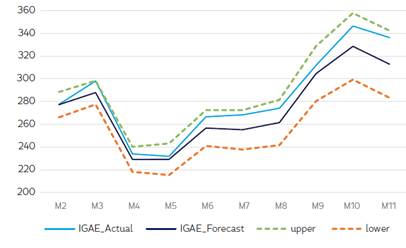
Considering models 1, 2 and 5 as the best models, it is possible to conclude that the mobility index and the individual grocery & pharmacy and workplaces change in visits relative to their baseline perform well in explaining the IGAE rate. The monthly and autocorrelation variables also show the importance of structural characteristics like patterns and built-in economic forces within the IGAE series in reproducing economic activity and growth, which, together with the mobility variables, do explain IGAE's behavior during 2020's COVID-19 first wave. Based on model 1, Figure 4 shows the actual behavior of the IGAE series during the COVID-19's first wave, together with the in-sample IGAE forecast within dotted 95% confidence intervals and a mean absolute percent error of 3,43. Both lines fall within the confidence intervals, indicating they are not statistically different.
5. Summary and conclusions
Attempting to establish the impact of the pandemic shock on economic activity from the perspective of its sources is a complex exercise. First, the COVID-19 policies tended to simultaneously include policies on many fronts, each with its specific impact on people's behavior and compliance. Second, COVID-19 has its own epidemiological dynamics that would operate differently everywhere depending on the initial conditions, among others. Third, The international context changed, affecting international mobility and trade. As this article argues, all of these constitute the pandemic shock that impacted the same population within a country, who had to make decisions and take actions to minimize health risks, subject to people's diverse economic circumstances and therefore subject to their willingness and possibilities for economic sacrifice. The latter is the channel that generated the secondary effect that impacted aggregate economic activity.
This article is about the connection between the people's behavior directly affected by the pandemic shock and how that behavioral change impacted indirectly aggregate economic activity. The Bolivian General Economic Activity Index (IGAE) produced by the National Institute of Statistics was the variable used to represent economic activity, and Google's COVID-19 Community Mobility Reports for Bolivia, which measure the percent drop in people's mobility concerning normalcy, was used as explanatory. It is argued that this explanatory captures the interactive impact of COVID-19 infections, COVID-19 policies, international restrictions, and population decisions regarding the balance between protection against health risks and economic sacrifice simultaneously.
The exploratory attempt is performed within an ARMAX modelling strategy. The model outcomes show that it is possible to conclude that the mobility data, particularly the changes in the rate of grocery & pharmacy visits, workplace visits and an aggregate mobility index, perform well in explaining the economic activity index rate changes. The seasonal and autocorrelation variables in the models also show the importance of economic structural characteristics and built-in economic forces within the IGAE series in reproducing economic activity and growth, which, together with the mobility variables, reproduce the economic activity index behavior during 2020. Complementary research should explore other modelling strategies to handle better time series at different frequencies, attempt to explain mobility in terms of the pandemic shock variables and improve causal inference.

