1. INTRODUCCIÓN

Underwater Vehicles have had great attention from industries due to their possibilities in naval operations for both, military and civil domains. The technological advances in this field allow them to be a useful tool for cost-effective deep underwater explorations, far beyond what humans are capable of reaching. They have been used for various missions such as inspection and survey, scientific underwater explorations, sampling and monitoring coastal areas, measuring turbulence and obtain related data, offshore installations and mining industries, military missions, among others. However, operation of a ROV in a vast, unfamiliar and dynamic underwater environment is a complicated process ¹.

The level of autonomy of the Autonomous Underwater Vehicles (AUV) is determined mainly by its performance in path planning and re-planning, being planning understood as the process of finding a trajectory that safely leads the AUV from its initial position to a target position. A large number of publications address the path-planning problem for AUVs. The reader can refer to the paper on ² for a broad review on this topic. The trajectory- planning problem has at least two components: the planner and the controller. The planner runs a tracker motion-planning algorithm, often expressed in an optimal frame, achieving a time-position trajectory to track. The controller drives the tracker to the specified trajectory positions ³. The trajectory-planning has to deal with decisions to maintain the trajectories that were planned by the mission control ⁴.

Real-life testing of both, planner and controller algorithms for trajectory-planning present a high risk of damage or even loss of AUVs if the algorithm fails, even if the testing is made on a controlled set-up environment. Therefore, it is necessary to substitute real-life testing with simulation, which is safer, and cost effective, avoiding on-board data collection, scenario construction and underwater recovery of AUVs. The work in ⁵ remarks these facts, and presents a review of graphical simulators for AUVs. The simulators can perform the job in different ways namely; offline, online, hardware in the loop (HIL) and hybrid simulation (HS), where real and virtual systems can function together in an improved environment. The more recently work in ² show a review about open-source developments for AUVs simulators, remarking that drawbacks of open-source developments are mainly the high learning curve for developers, and the difficulties to emulate the hydrodynamics forces interacting with the AUV.

MSC ADAMS®, and MatLab® are commercial software packages widely used for the scientists around the world. MSC ADAMS software is intended for Automatic Dynamic Analysis of Multibody Systems and it provides a great suit of tools for building virtual environments composed of 3D objects, being compatible with specialized CAD software such as SolidWorks. The motor of physic of MSC ADAMS allows the user the settling of properties such as gravity, 3D forces and wrenches, torques, materials of bodies, and so on. A variety of physical measurements for variables and actuators are available in MSC Adams allowing comprehensive analysis of system by using a simple and flexible modeling of solid objects. These objects are then interconnected by means of kinematic links and movement constraints into a single unit, which corresponds to the real characteristics of the mechanic system ⁶. The MSC ADAMS controls tool allows exporting the computed dynamic model to MatLab. The co-simulation property implemented in MSC ADAMS allows the exchanging of information between the two simulators at simulation time, so the user can take advantage of the remarkable capabilities of MatLab for analysis and design of controllers in order to control the ROV/AUV system. Some works reported using MSC ADAMS and Matlab in co-simulation are ^{7), (8), and (9}, demonstrating its potential for simulation of mechanical dynamic systems.

This work explores the feasibility of using Mat-Lab and MSC ADAMS in co-simulation for building virtual environments intended for analysis and design of trajectory tracking controllers for ROV/AUVs. Remarkable properties derived of the use of these commercial software are: low virtual environment development time, easy modeling of hydrodynamic forces, realistic dynamic behavior without the needing of complex theoretical developments, and direct availability of signals on the MatLab simulator for both, analysis and control design purposes.

2. MATERIALS AND METHODS

The procedure for building and validating the virtual environment is:

To validate the aforementioned procedure, in this work a simple environment was implement in MSC ADAMS/View consisting of:

Definition of the materials for each body in the MSC Adams model are necessary in order to enable dynamic simulations. The main advantage of using ADAMS is that the geometric models of solids are sufficient; the program will automatically calculate the movement of the whole system in pursuance of individual members, which are prescribed by movement or by force application. Thrusters were simulate by mean of two orthogonal single forces.

Source: The authors.

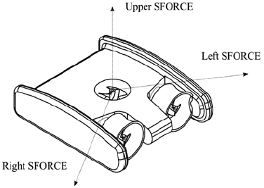
Fig. 1. DISPOSITION OF THE MSC ADAMS FORCES USED TO SIMULATE THE RESULTANT FORCE OF THRUSTERS MOVING THE ROV 

(SFORCE) disposed symmetrically to the central axis of the ROV in the plane parallel to the subsea surface (horizontal plane) and a third orthogonal single force was dispose in the normal plane to the subsea surface (normal plane), as is it shown in Figure 1. The resultant force of the three thrusters allow the movement of the ROV in the horizontal plane and in the normal plane. The vectors of these three orthogonal forces were align to be coincident with the center of mass of the ROV/AUV.

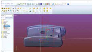
Hydrodynamic forces of the sea interacting with the ROV were simulated by mean of a general force (GFORCE) attached to the center of mass of the ROV. The GFORCE has six general force components, three for the translational force and three for the torque. Position measurement provides the three translational components of the ROV center of mass, and orientation measurement provides the three orientation angles of the ROV center of mass. Figure 2 shows the Adams/View implementation of the virtual environment for the simulation experience.

Source: The authors.

Fig. 2. VIRTUAL ENVIRONMENT FOR THE SIMULATION EXPERIENCE IN MSC ADAMS/VIEW 

Port inputs for the Adams model correspond to the modeled forces, whereas port outputs of the Adams model correspond to the measures. With these defined ports, the tool ADAMS/Controls can export either a linear or a nonlinear dynamic model for the MatLab program. The nonlinear model is a better approximation for the system; and it is created as an s-function for MatLab. Figure 3 shows the Simulink block for the s-function based model of the ROV.

Source: The authors.

Fig. 3. EXPORTED MASKED S-FUNCTION FROM MSC ADAMS FOR THE SIMULINK ENVIRONMENT 

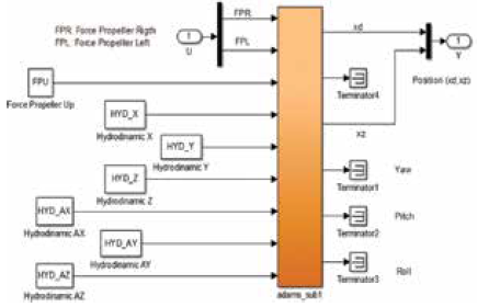
Details about how to generate the Adams_sub block for co-simulation in Figure 3, how to use Adams/ Control to export the s-function, and how to configure the Simulink block for co-simulation are beyond the scope of this paper. However, there are a lot of available tutorials and papers describing these procedures. The interested reader can review the MSC Adams guide in ¹¹ for details.

The trajectory-tracking experience chosen in this work consists in evaluating the performance of a LQR based controller for tracking position zig-zag and circular trajectories in the horizontal plane, as they are usually employed by researchers in this kind experiments with ship model ^{12), (13), (14), (15}, for the horizontal plane. To these ends, a linear model for the system must be computed. The linear model computed by MSC Adams usually is not a good selection for control design purposes since dynamical effects of external disturbances are not taken into account, besides the ignorance of an adequate operation point for the problem. A better procedure is to build an experiment in MatLab, taking into account variations on the inputs of the system exiting the dynamic behavior of the controlled variables, and computing a linear model by mean of its identification toolbox. Since this experience evaluates just the movement in the horizontal plane, the identified model has two manipulated input variables, namely, the Propeller Right Force component (FPR), and the Propeller Left Force component (FPL). The Propeller Up Force (PFU), it only has a constant value of zero because the horizontal plane is not evaluated. Propeller forces are those forces that are obtained by the propulsion of displacement between the dynamics of the propeller and the water that causes a push or step from the static state to the dynamic state or movement.

On the other hand, there are three measured disturbance inputs, namely, the hydrodynamic translational force components in the horizontal plane (HYD_X and HYD_Z), and the hydrodynamic torque component around the normal axis to the horizontal plane (HYD_AY). These hydrodynamic forces in the horizontal plane are constant; this is because the hydrodynamic forces are exerted on the surface of the ROV producing opposition to the movement in the form of a flow influencing the acceleration and navigability of the ROV. As the ROV displacement has slow speed an acceleration, the hydrodynamic forces are very close to zero within this study; however, they can be replaced by any time function created by MatLab. Measured output variables (controlled variables) are the center of mass, whose components in the horizontal plane are CM_X and CM_Z. The center of mass position is very related to the buoyancy of the ROV.

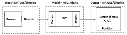
A co-simulation experiment was conducted where exciting input vector of forces were computed in the MatLab software, sent them to Adams/ View to compute the resultant dynamic behavior of the center of mass position, and retrieved again to MatLab to obtain the measured output vector of positions. Figure 4 illustrates the above-mentioned co-simulation schema. By mean of the graphic user interface of the identification MatLab toolbox, a 4th order linear state space model was compute from the input and output vectors collected during the simulation time.

Source: The authors.

Fig. 4. SISTEMA DE NAVEGACIÓN DEL RUMBO EN EL PLANO HORIZONTAL 

The following steps carried design of the trajectory tracking LQR based controller from the identified linear model.

There are several solutions proposed before in the literature for the tracking of position trajectories problem using the LQR approach, see ¹⁶ for an example. They can go from the classic plant augmentation with an integral action, the building of a trajectory generator model for plant augmentation, to the estimation of a model for the disturbances. In this work, the simplest robust LQR with integral action approach is used in order to evaluate the proposed virtual environment. Since the identified linear model is defined on arbitrary and unknown state variables, a state observer is needed in order to be able of apply an LQR approach from the measurements vector. Control theory for linear observer design and LQR design for plant augmentation with integral action are very known approaches described in almost any modern control textbook.

3. RESULTS AND DISCUSSION

3.1 Identification of ROV model without disturbance

The representation for the ROV dynamics is an invariant time (LTI) state space model of in the standard form of the equation 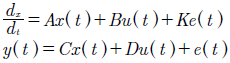(1).

(1)

Where A, B, C, D and K are suitable matrix of constant parameters,u = [FPR, FPL] ^T  is the vector of manipulated propeller forces (input),y = [CM_X, CM_Z] ^T is the vector of position components of the center of mass (output) with unids in meters, x is the state vector, and e is the state disturbance vector.

The identification was performe by mean of the ident function from the MatLab identification toolbox, yielding to the following matrices:

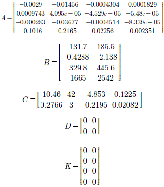
By providing forces in the propellers (Propeller Force Right [FPR] and Left [FPL]) an ROV shift is obtained, carried out in the virtual environment in ADAMS without any automatic control action; where the ROV is followed by the change of position of the center of mass. It is clear that the center of mass of the ROV does not change, it’s only observed as the position of that center of mass moves from one place to another within a space. (Showed in the Figure 5).

Source: The authors.

Fig. 5. DISPLACEMENT OF THE ROV BY TRACKING THE CENTER OF MASS 

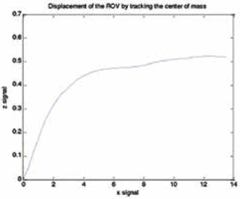
Figures 6 show the output position components of the center of mass, comparing the output of the nonlinear model computed by Adams, with the response to the same inputs of the LTI state space model identified. The median square error (mse) for the component CMx is 0.0381 percent, while the mse for the CMz component is 0.0403 percent, which indicates that both CMx and CMz predicted by the LTI model are good enough for controller design purposes.

Source: The authors.

Fig. 6. COMPARISON OF THE POSITION OF THE CENTER MASS IN CMZ Source: The authors. 

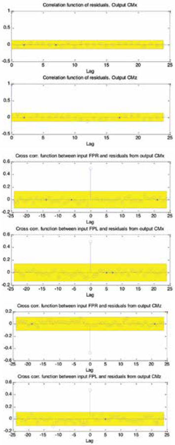
The residual correlation function between CMx, CMz, FPR and FPL are all within the Bartlett bands or 99% confidence zone for all delays, using the Matlab resid (ss1, datROV) statement. This statistical notation indicates that the identified model describes the real system accurately and any control design will offer a good control capability even if there are delays between the input signal (FPR and FPL) and the output signal (CMx and CMy) when the identified model is implemented within the virtual environment of MSC ADAMS. Therefore, this shows that the identified model is correct. (See figure 7).

3.2 LQR controller design with Observer and with integral action

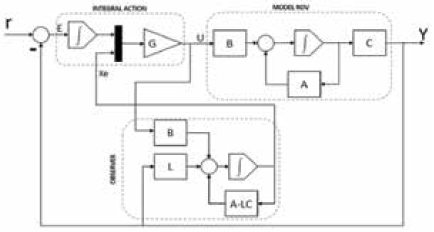
Figure 8 shows the implemented control strategy for position tracking evaluation purposes. The LQR controller is a state feedback based approach, being G the feedback gain. However, the four identified states are physically meaningless; therefore, a state observer is mandatory in order to estimate the state from the measured outputs. The identified model fulfills both, the observability and controllability properties.

Source: The authors.

Fig. 7. THE CORRELATION FUNCTION OF RESIDUALS: CMX, CMY, FPR, FPL 

Integral action is required in order to minimize the steady-state position error and constant or slow disturbances ^{17), (18}. Plant augmentation with the integral of the tracking error is a common procedure used for design purposes, this illustrated in the Figure 9, where the feedback gain matrix is applied to the augmented state.

Source: The authors.

Fig. 8. LQR WITH OBSERVER AND INTEGRAL ACTION AUGMENTATION SCHEMA 

The optimization function J was define as the infinite time horizon function, where is the state vector augmented with the two components of the integral position error of the center of mass. The augmented state weight matrix is a matrix of ceros except for the diagonal terms weighting the integral of the position error, which were settle to one. The input weight matrix is the identity matrix pre-multiplied by the one degree of freedom positive constant design parameter. Then, the state feedback gain can be solved by the MatLab sentence: G = lqr(Aa,Ba,Q,R), being Aa and Ba the augmented matrices resulting of the augmentation process. was the design parameter which yields to a good balance between error a control effort performance. In the other hand, the observer gain can be computed by a pole placement assignment algorithm ensuring the matrix, being Hurwitz and the observer poles faster than those of the controller closed loop. These procedure can be achieved using the MatLab sentence L=- place(A’,C’,P)’, where A and C are the state matrices and P is a vector with suitable desired poles.

This work doesn’t emphasize on the resulting performance of the designed controller, it just presents the possibilities of Admas-Matlab co-simulation for the design and validation of trajectory position controllers for a ROV. As a reference for further reading about LQR for position trajectory tracking control, the work of Fossen in ¹⁶ shows a general solution for the design of the trajectory tracking problem based on LTI models, which proposing a LQR controller suitable for disturbance rejection thorough a disturbance estimation model.

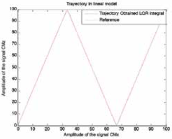
Figure 9 shows a zig-zag trajectory reference and the resultant output position tracking for the center of mass in the X-Z plane obtained from Simulink with the identified dynamic LTI model, without the Adams model. The objective of this experiment is the parameters adjustment of the controller and observer in the control scheme.

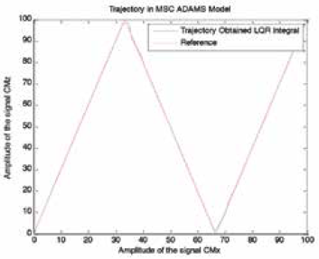
The tracking results of Figure 10 correspond to the same reference signal but now using the Admas- Matlab co-simulation in Simulink. Very close results respect to the LTI performance indicate a good performance of the control strategy.

Source: The authors.

Fig. 9. TRAJECTORY TRACKING PERFORMANCE USING THE IDENTIFIED LTI MODEL FOR CONTROLLER VERIFICATION 

Source: The authors.

Fig. 10. TRAJECTORY TRACKING PERFORMANCE USING THE VIRTUAL ENVIRONMENT BASED ON ADMAS-MATLAB CO-SIMULATION 

3.3 Simulating a surf effect as a disturbance source

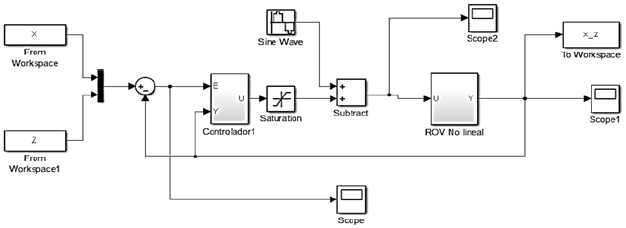
Besides the possibility of using the hydrodynamic forces disposed in Adams as a source of disturbances, some disturbances can be modeled directly from the Simulink model. Figure 11 shows the Simulink model for an experiment where the oscillatory behavior of waves on surfing were suppose being additive disturbance to the propeller forces as in ^{19), (20}. The sine block in the Simulink model of Figure 11 was dispose for this end.

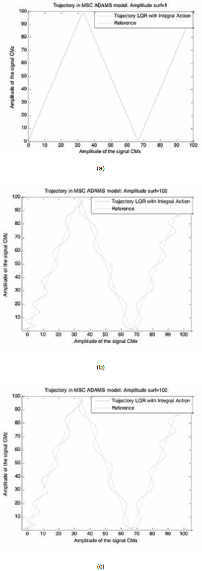
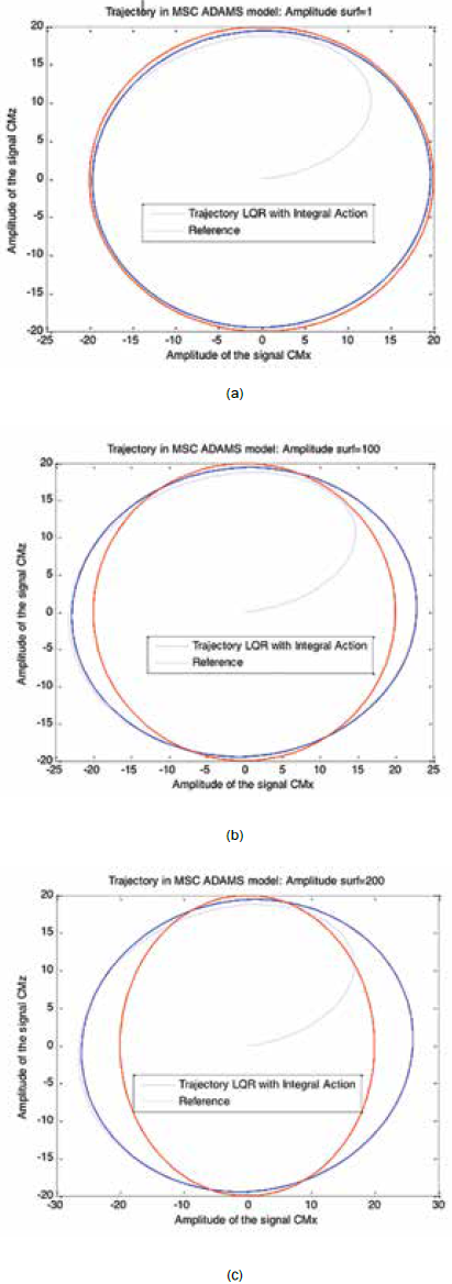
Figure 12-13 shows the trajectory tracking performance resulting of the experiment for three sine amplitudes, namely, 1, 100 and 200; all with frequency of 1 Hz. Figure 12-13 a) shows an acceptable performance for disturbance rejection despite of the simplicity of the control approach. Figure 12-13 b) and c) shows how a better disturbance rejection strategy needed for large disturbance forces. This kind of control performance evaluation is feasible for the Adams-MatLab co-simulation virtual environment without a great development effort.

The previous experiments, despite the simplicity of the control strategy and the non-existence of an adequate study of the hydrodynamic forces of the environment, they have allow to explore the efficacy of the proposed method for building virtual environments for ROV position controller design and evaluation. A list of the summarizing skills of the Admas-MatLab co-simulation procedure for that purpose is:

• Easy importation of CAD 3D models to MSC ADAMS for the ROV structure in several formats such as: Iges, Parasolid, Solid Works assembly.

• Possibility of attaching generalized forces (with six spatial components) to nodes of the ADAMS model of the ROV in almost any place of the structure, simulating either propulsion forces or hydrodynamic forces.

• Easy building of a realistic dynamic model compatible with MatLab-Simulink without the needing of any theoretical development exploding the capabilities of the Adams Control tool.

• Possibility of simulating contact forces, gravity, and other physic mechanic behavior.

• Availability of easy access to signals from sensors or toward actuators from MatLab-Simulink model in simulation time.

• Availability of the high power of MatLab tools for control and system identification.

• Communication between MSC Adams and MatLab is a no time consuming process for developer and it has been well described in literature internet available tutorials.

• The ROV movements can be visualized in the 3D virtual environment, besides the measured signals using the co-simulation property of MSC Adams.

The Adams-MatLab co-simulation advantages for controller design and identification, allows other kind of approaches useful in this control problem such as:

• Building of an analytical model for the ROV using the Lagrange approach of other mathematical tools, and performing a parameter matching from the Adams nonlinear s-function in order to have a nonlinear dynamic model allowing nonlinear control techniques such as feedback linearization based controllers, sliding mode control, among others.

• Researching about realistic models taking into account the specific materials properties of the ROV, modeling of hydrodynamic forces matching some sea conditions, etc.

• Testing the effect of additional propellers in another positions or orientations.

Source: The authors.

Fig. 11. SIMULINK MODEL FOR EVALUATION OF THE CONTROL STRATEGY IN PRESENCE OF OSCILLATORY DISTURBANCE 

Source: The authors.

Fig. 12. TRAJECTORY TRACKING PERFORMANCE USING THE VIRTUAL ENVIRONMENT BASED ON ADMAS-MATLAB CO-SIMULATION INCLUDING A SURFING EFFECT. A) SINE AMPLITUDE = 1, B) SINE AMPLITUDE = 100, C) SINE AMPLITUDE =200 

Source: The authors.

Fig. 13. TRAJECTORY IN MSC ADAMS WITH A) SINE AMPLITUDE = 1, B) SINE AMPLITUDE = 100, C) SINE AMPLITUDE = 200 OF AMPLITUDE THE DISTURBANCE 

CONCLUSIONS

This work has shown a procedure for the building and validation of virtual environments for ROVs position tracking based on co-simulation between MatLab-Simulink and MSC Adams. Remarkable advantages of these procedures have been listed as a discussion of the simulation results. Despite the simplicity of the chosen control strategy for trajectory position control of the ROV, and despite the non-existence of a realistic study for emulating the hydrodynamic forces, the obtained results show the potential of this procedure for more complex and detailed modeling skills in this field. Future works should take advantage of the proposed generalized forces tool in order to matching actual prototype buildings with hydrodynamic and propulsion forces in a controlled environment, and to identify realistic disturbances and problems yielding to formulate a more complex control structures to solve these problems.