ORIGINAL ARTICLE

ESTIMATION OF NEURONAL ACTIVITY AND BRAIN DYNAMICS USING A DUAL KALMAN FILTER WITH PHYSIOLOGYCAL BASED LINEAR MODEL

ESTIMACION DE LA ACTIVIDAD NEURONAL Y LA DINAMICA DEL CEREBRO USANDO UN FILTRO DE KALMAN DUAL BASADO EN UN MODELO FISIOLÓGICO LINEAL

^* Profesor asistente. Programa de Ingeniería Eléctrica, Facultad de Ingenierías, Universidad Tecnológica de Pereira. Vereda La Julita, Pereira. E-mail: egiraldos@utp.edu.co

^** Profesor titular. Programa de Ingeniería Electrónica, Facultad de Ingeniería y Arquitectura, Universidad Nacional de Colombia, sede Manizales. E-mail: cgcastellanosd@unal.edu.co

Recibido: 26/01/2012

Aceptado: 07/05/2013

RESUMEN

In this research article a dynamic estimation of neuronal activity and brain dynamics from electroencephalographic (EEG) signals is presented using a dual Kalman filter. The dynamic model for brain behavior is evaluated using physiological-based linear models. Filter performance is analyzed for simulated and clinical EEG data, over several noise conditions. As a result a better performance on the solution of the dynamic inverse problem is achieved, in case of time varying parameters compared with the system with fixed parameters and the static case. An evaluation of computational load is performed when predicted dynamic cases, estimated using the Kalman filter, are up to ten times faster than the static case.

PALABRAS CLAVE

Inverse problem, Kalman filter, estimation, physiological model, brain model.

ABSTRACT

En este artículo de investigación se presenta la estimación de la actividad neuronal y la dinámica del cerebro a partir de señales electroencefalográficas (EEG) usando un filtro de Kalman dual. El comportamiento dinámico del cerebro se representa a partir de modelos lineales con base en restricciones fisiológicas. Como resultado, se obtiene un mejor desempeño en la solución en el caso de modelos variantes con el tiempo, al compararla con modelos invariantes en el tiempo, y con la solución estática. Se presenta una evaluación de la carga computacional donde es claro que la estimación de la actividad neuronal con el filtro de Kalman basada en modelos dinámicos lineales, es hasta 10 veces más rápida, que la solución para el caso estático.

KEY WORDS

Problema inverso, filtro de Kalman, estimación, modelo fisológico, modelo del cerebro.

INTRODUCTION

Functional neuroimaging aims to non-invasively characterize the dynamics of the distributed neural networks that mediate brain function in healthy and pathological states. As rule, neural current distribution within the brain or neuronal activity is estimated through functional Magnetic Resonance Imaging (fMRI) or electroencephalographic signals (EEG). Former technique allows direct estimation of neuronal brain dynamics with high spatial resolution, but providing low temporal resolution. On the contrary, the images generated by EEG inverse solutions exhibit a lower spatial resolution, but possess a much higher temporal resolution, which is important for studying brain dynamics [1]. In this regard, since the neuronal activity has an inherent strong spatial and temporal dynamics, the source localization task (the inverse problem) instead of being calculated using only the measurement at one single time point might consider the dynamic variability of the neuronal activity [2]. In other words, the inverse problem should include dynamic constraints that take into account the evolution of the neuronal activity, by choosing appropriate dynamical models [3].

Nonetheless, several issues need to be considered for the dynamic inverse solution. The main restriction is the selection of the dynamical model. According to [4, 5], linear or nonlinear dynamic models should be considered as an approximation of brain dynamics. This incorporation of physiological meaningful models into inverse solution framework can provide a better description of the system dynamics. For example, linear models of first and second order with time invariant parameters are employed in [1, 6], but these approximations only can track simulated EEG signals, even when these are physiological meaningful models. Consequently, for real EEG signals, some variants of the dynamic model should be considered in order to improve the performance of the dynamic model for spatial and temporal behavior, such as more complex linear or nonlinear models, and temporal variability for the source and local neighbor interaction.

Besides, dynamic neuronal activity estimation is a high dimensional task and its implementation leads to exasperating computational load. In this line, Kalman filtering is discussed in [6] as an alternative that includes a decoupling of the dynamic model for each source independently reducing computational load. However, when dynamic model performance is evaluated over real EEG signals they obtain problems in spatial coupling as a result of the decoupled implementation. So, it is possible to improve the performance of the decoupling method proposed in [6] using methods of filter partition [7] or high performance computing [8].

This article presents an estimation method for neuronal activity on the brain, taking into account in the solution of the inverse problem a dynamic model with time varying parameters. This model is applied over a realistic head model calculated with boundary element method. The analysis is made up from simulated EEG signals for different levels of noise. The solution of the inverse problem is achieved using high performance computing techniques by Kalman filtering methods where neuronal activity and model's parameters are estimated simultaneously. This article is organized as follows: section 1 presents models for solving the inverse problem for the static and dynamic case using Kalman filter for estimation of neuronal activity and model parameters. Section 2 shows a head model using boundary element method (BEM) and section 3 develops the comparative analysis between the static and dynamic methods for several noise conditions in case of simulated and clinical EEG signals with superficial and deep sources.

1. MATERIALS AND METHODS

1.1 Inverse problem framework

Solution of the inverse problem using distributed sources presents a high computational load, for that reason, in [8] high performance computing (HPC) techniques are used for the development of the solution in dynamic inverse problems. Estimated neuronal activity will be mapped over a realistic head model obtained from fMRI. Realistic head models will be used for analysis according to [3, 2, 6].

The static inverse problem can be formulated as follows

In equation (1), y_k denotes a vector of dimension d × 1 that contains the measures of the EEG on the surface of the head for d electrodes in an instant k of time. x_k = [x^T₁ ... x^T_N]^T denotes a 3N × 1 vector that contains the current density vectors x_i = [x_ix x_iy x_iz]^T with i = 1, 2, ..., N where N is the number of sources inside the brain. Matrix M has a d × 3N dimension and it relates the current density inside the brain x_k in instant k with EEG measures y_k. It is called lead field matrix and can be calculated using Maxwell equations for a specific head model [2]. The vector ε with d × 1 dimension is an additive random variable that represents the non-modeled features of the system, i.e. observation noise, and it can be assumed as a Gaussian distribution of the form ε ˜ G(0,σ²∑_ε) with known covariance structure ∑_ε.

This is an ill-posed problem and the estimation of can be obtained by minimizing the objective function given in equation (2) for each time k independently.

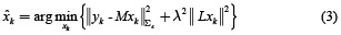
where L is defined as the spatial smoothness constraint where the ith row vector of L acts as a discrete differentiating operator (Laplacian operator) by forming differences between the nearest neighbours of the jth source and ith source itself. The parameter λ, called regularization parameter, expresses the balance between fitting the model and the prior constraint of minimizing Lx_k. It can obtain an estimate of by minimizing equation (2), as given by equation (3).

The solution of this minimization problem for a given λ is obtained by equation (4).

The parameterλ is calculated using methods of parameter selection as L-curve [9].

The dynamic inverse problem sustains the same equation for measurements observations but takes in to account the dynamic of the neuronal activity x_k, this problem can be formulated as follows

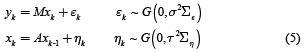
where A is a matrix that takes into account the dynamic of the neuronal activity, and ∑_η = (L^TL)^–1 is a covariance matrix associated with _η.

The structure of A is selected according to a physiological based model proposed by [5, 6]. In the case of a first order linear model x_k = Ax_k–1 + _k, A is defined as follows

where a₁ considers the variability among sources in time and b₁ in space.

Moreover, in order to consider a more realistic dynamic [5], the state equation presented in (5) could be extended to a second order linear model given by equation (7)

where

This model can be formulated in the form of a first order model as follows

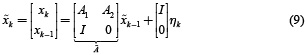
with

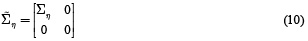
Therefore, equation (5) with the structures given by equations (6) and (9) is an ill-posed inverse problem and can be solved by minimizing the objective function given in equation (11)

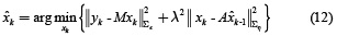
An initial estimate (for k = 1) of the state x₁ can be obtained by any approach for solving the instantaneous inverse problem. For k = 2, ..., N, we can obtain an estimate of by minimizing equation (11), as given by equation (12).

where is the estimate obtained in the previous step. The solution of equation (12) is given by (13).

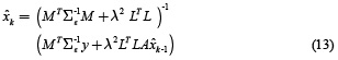
Direct computation of this expression is numerically impracticable because the inverse of dimensions of M. However, the dynamic inverse problem in case of neuronal activity estimation x_k presented in equation (13) is a state space formulation that could be solved through the Kalman filter.

1.2 Neuronal activity estimation

Kalman filter recursions in case of states (neuronal activity) estimation are given by the equations (14) and (15).

Equation (14) is known as time update equation

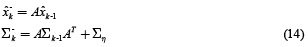
where is defined as a priori estimation of , and is defined as a priori covariance.

The measurement update equations for the state filter are

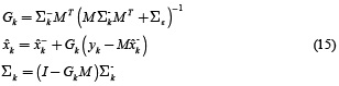
This formulation is useful if A is considered as a fixed matrix for all k.

1.3 Neuronal activity and parameter estimation

In order to achieve an improvement in the dynamic model is useful to consider A as a time varying matrix A_k for each k. Consequently, the solution of the dynamic inverse problem in case of neuronal activity estimation x_k and parameter estimation A_k could be formulated using two sequential Kalman filters given by the recursion presented in equations (16) – (19).

Time update equations for parameter filter are

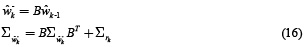
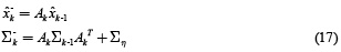
And those for the state filter are

The measurement update equations for the state filter are

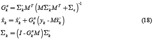
And those for the parameter filter

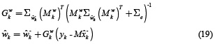
where is defined as a vector that contains the coefficients a₁, b₁ of equation (6), or coefficients a₁, b₁, a₂ of equation (8). 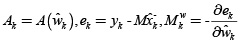, ∑_e is the associated covariance matrix of e, B is the structure of time varying parameters (specifically, for this work B = I for random walk), and is the covariance associated with the parameter variation. This estimation is known as a dual Kalman filter.

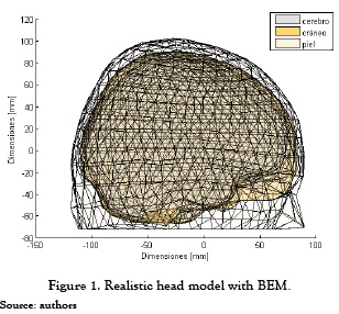
1.4 Head modeling through BEM

In head modeling there can be used from simple models such as spherical, to complex models like finite elements, boundary element method, finite volumes, finite differences, etc. Modeling with the boundary element method (BEM) presents a middle point of complexity between the named models, obtaining a more realistic approximation of the head model while it keeps some properties of simple spherical models (i.e. uniform conductivity). The head models vary their complexity with the number of layers, like follows: a layer: the brain; two layers: brain and skull; three layers: brain, skull and skin; four layers: brain, skull, cerebrospinal fluid, skull and skin [3].

The BEM model consists of a set of point located over every layer of head model and that form the vertices of a set of triangles. This way, the realistic model obtained corresponds to an approximation through the set of triangles for every layer which are considered isotropic conductivities in the same way as is done for the spherical model.

Thus, the lead field matrix M involves spatial relationships between sources located within the brain (inner layer) with located electrodes over the skin (outermost layer). Figure 1 shows the head model with three layers using BEM.

2. RESULTS AND DISCUSSIONS

Initially, system dynamics will be approximated through a linear time invariant model. This linear model must consider temporal and spatial constraints of dynamical process. In order to improve dynamic model performance, structural model variations that preserve spatio-temporal constraints will be considered. For neuronal activity approach, a linear time invariant physiological based model will be used according to [5] that take into account anatomic constraints related with spatial coupling between sources. According to [1, 6], structural changes of linear dynamic models will be analyzed, considering physiological constraints in a time invariant model. Then, an evaluation of the performance of dynamic models proposed by [6] will be used for the different applied models considering principally estimation error in simulated a real EEG signals.

Since real dynamical models are time varying, an estimation of dynamic model parameters will be developed, consistent with the different structures for parameter variation as proposed by [10]. In each case, the methodology for dynamic inverse problem solution proposed in [6] will be used for estimation of neuronal activity considering error estimation in simulated EEG signals. A comparative analysis will be performed among different dynamic models with applied variation structures and with fixed parameters, using simulated EEG signals. A schematic diagram of the experimental setup is presented in figure 2.

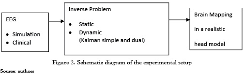
2.1 Experimental setup

In order to obtain the dynamic estimation of neuronal activity and brain dynamics using a physiological based linear model, the Kalman filter and dual Kalman filter are applied to EEG data. To consider the relative contribution to the filter performance of different parts of the process model for the dynamic inverse problem, in case of a first and second order linear system and its comparison with the static inverse problem, the following cases are to be considered: 1) static case of equation (1); 2) first order model given in equation (6) with fixed parameters without spatial coupling (b₁ = 0); 3) first order model with spatial coupling with fixed parameters; 4) second order model of equation (8) with spatial coupling with fixed parameters; 5) first order model with adaptive parameters without spatial coupling (b₁ = 0); 6) first order model with spatial coupling with adaptive parameters; and 7) second order model with spatial coupling with adaptive parameters.

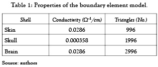
Testing is carried out for simulated and clinical EEG recordings, as well. Prior to computing an inverse solution, we define a discretized solution space consisting of 7x7x7 mm gray matter grid points (sources), as recommended in [6]. These sources cover the cortex and basal ganglia. At each source, the 3D local current vector is mapped, as usual, to the 19 electrode sites for the 10 - 20 system. The properties of the BEM model used for brain mapping are shown in table 1.

Finally, an evaluation of the computational load is performed for static case over first order and second order linear dynamic cases, using simple and dual Kalman filter.

2.2 Simulated EEG recordings

A major issue regarding to the inverse solution task is obtaining meaningful evaluations of the algorithm's results and performance, because location of true sources is not available for comparison when working with real EEG data. Instead, the most common approach is to use simulated EEG data where underlying sources are known. Two types of sources will be used: sources randomly located near the surface of the brain and sources randomly located deep in the brain. Nonetheless, to generate a simulated EEG dataset for this purpose requires selecting a model for the brain dynamics, which displays complex spatio-temporal behavior. Here, the temporal dynamics are suggested to be modeled using a linear combination of three sine functions whose components are evenly spaced in the alpha band (8-12 Hz), which is selected since the clinical data used in real EEG recordings display prominent alpha activity [6]. Specifically, the simulated brain dynamics where generated for 256 time points, assuming a sampling rate of 256 Hz.

The performance of the inverse solutions is compared with simulated EEG data for the following values of SNR: 5 dB, 10 dB, 15 dB, 20 dB and 25 dB for each type of source. Besides, 25 repetitions of one second of synthetic EEG data, according to 10 - 20 system, are generated from the simulated current densities by multiplication with the lead field matrix M.

The obtained results for the static case solution of equation (1) when considering several SNR are shown in table 2, where a regularized solution is used to solve the inverse problem of equation (3). In this case, a Tikhonov solution with L-curve method for parameter selection is used [9]. It can be seen that the obtained results are similar to the outcomes given in [2], namely, the performance of the considered algorithm is highly dependent of the noise.

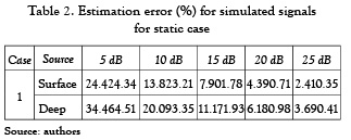
On the other hand, when temporal constraints are included in the solution of the inverse problem, the solution of the inverse problem could be improved. Nonetheless, it is shown that if choosing appropriate dynamic models, better solutions than those obtained by the static case can be achieved [1].

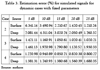
In the case of a dynamic model with time invariant parameters, when assuming first and second order models, the obtained results are shown in table 3, which are similar with those outcomes given in [6], for time invariant parameters (calculated offline). For example, when looking to the first order model without spatial coupling (i.e. case 2), the results are not as good as in the case of the first order model with spatial coupling (case 3); whereas the second order model shows better performance in case of dynamic estimation with fixed parameters. It must be quoted that similar result, for the considered variations of the dynamic model, where obtained in [6]. Nonetheless, the main drawback of a time invariant model is that in case of any model change, the estimation error significantly increases.

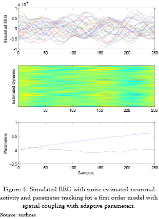
As shown in figure 3, the estimated neuronal activity of each source vs. samples, when considering the static inverse problem (middle subfigure), is highly dependent of the level of noise. On the opposite, estimated dynamic solution (bottom subfigure) that takes into account the noise variability shows a better approximation of original activity (upper subfigure).

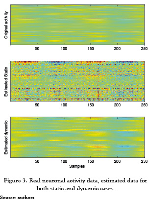
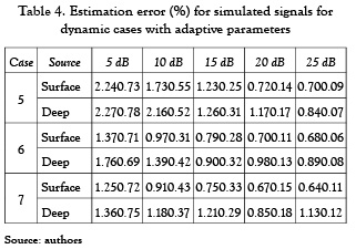
Table 4 resumes the obtained results for dynamic models with time variant parameters, given by first and second order models with spatial coupling of Equations (6), (8) respectively. It can be seen clearly that for time variant parameters, a lower estimation error in presences of high noise is achieved, since the estimated model takes into account the variability of the signal. Moreover, the best performance is achieved using the second order model with time variant parameters. As a result, even that the lead field matrix M is fixed any occurred change either in the conductivity of the brain or external stimulus is considered as a variation into the whole assumed adaptive model.

As illustration, the EEG data with noise, the dynamic solution of a first order model with spatial coupling (case 6), and the parameter progress are shown in figure 4 with a 15 dB SNR. Hence, the time variant parameters shows convergence in the case of spatial coupling, around b1=0.01, whose value is some close with the results estimated by [6], when offline parameters is appraised. This behavior of parameters points out on the necessity to consider the spatial coupling in the model even when if their values might be considered small in comparison with ones of the temporal behavior, as discussed in [11].

2.3 Clinical EEG recordings

In case of real EEG signals we now estimate inverse solutions for a time series chosen from a normal EEG recording collected during routine clinical practice (Neurocentro de Occidente, Pereira, Colombia). The data were recorded from a healthy male adult aged 45 years, in awake resting state with eyes closed. Electrodes were placed according to the 10–20 system and the data were collected at a sampling rate of 256 Hz. The resolution of the AD conversion was 12 bit. A 2 seconds time series was selected from the recording for analysis.

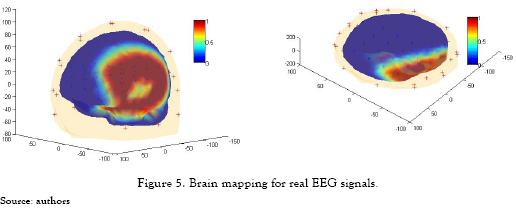
A dual Kalman filter with a second order model is used for real EEG signals in case of an eyes closed event. The estimated neuronal activity spatially localized is mapped over a realistic BEM head model, as shown in figure 5. Here, an area of activity is presented at the right occipital pole as expected for prominent occipital alpha activity. These observations are consistent with an eyes–closed event in EEG recording.

2.4 Computational load

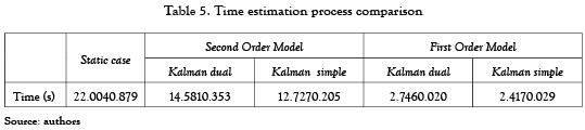
In order to evaluate the performance of the solutions from a computational load point of view using the high performance computing techniques, an evaluation of the estimation process time is performed for static case, first order and second order linear dynamic cases using simple and dual Kalman filter. This analysis is performed over a single computer with dual core of 2.6 GHz processor and 2 GB of RAM. In order to address the limitation of large scale computations, we arrange the Kalman filtering computations such that the data intensive aspects of the algorithm can run in parallel. The results of this evaluation for 25 repetitions of each case are shown in table 5.

It is noticeable from table 5, that the time of estimation for the dynamic cases of the first order model is 10 times less than the static case. In particular, the estimation time of the second order model requires 5 times more than the first order model because the formulation of the model is according to equation (11) which duplicate the number of sources of the linear model. Even so, the second order model requires almost the half of time than the static case.

3. CONCLUSIONS

In this paper, we have addressed the dynamical inverse problem of EEG signals for estimation of neuronal activity and brain dynamics, being a generalization of the more traditional instantaneous and dynamic inverse problems, and we have presented a new approach for estimating the time varying parameters of the dynamic model itself. The obtained results demonstrate that the model with adaptive parameters has a better performance than the instantaneous inverse problem and the dynamic inverse problem with fixed parameters. This improvement is because the model with time varying parameters takes into account any variation of the brain dynamics.

If only a very simple model is employed, the resulting inverse solution may not offer much improvement over the results provided by instantaneous techniques. As expected, the more elaborate a dynamic model is applied, the more the resulting inverse solutions will be able to explain the observed EEG data. These results were confirmed for each case study in this paper for simulated signals over several SNR values where the second order model with adaptive parameters reached the better performance. In general, the dynamic models with adaptive parameters for neuronal activity estimation shows a better performance over signals with low SNR values in comparison with the models with fixed parameters and the instantaneous case.

Additionally, in real EEG signals the estimated activity may be particularly useful for localizing points or areas within brain that display typical or atypical behavior, such as epileptic foci or others events.

Furthermore, there is a relevant reduction in the computational cost for the dynamic cases over the static case even for the second order linear model which is the most critical case because duplicate the number of sources. In case of the first order linear case the reduction of time for the dynamical calculations is less than ten times the static case. Consequently, the dynamic implementation of the Kalman filter applying high performance computing techniques reduce the computational cost and facilitate large scale calculations.

For future work, more complex dynamic models (such as nonlinear models) should be calculated in order to improve the performance of the estimator.

4 ACKNOWLEDGMENTS

Authors would like to thank COLCIENCIAS for the financial support on the project ''Sistema de Identificación de Fuentes Localizadas Epileptogénicas Empleando Modelos Espacio Temporales de Representación Inversa''.

REFERENCES

[1] O. Yamashita, A. Galka, T. Ozaki, R. Bizcay, and P. Valdez-Sosa, ''Recursive Penalized Least Squares Solution for Dynamical Inverse Problems of EEG Generation'', Human Brain Mapping, vol. 21, pp. 221-235, jul., 2004.         [ Links ]

[2] R. Grech, C. Tracey, J. Muscat, K. Camilleri, S. Fabri, M. Zervakis, P. Xanthoupoulos, V. Sakkalis, and B. Vanrumste, ''Review on solving the inverse problem in EEG source analysis'', J. of NeuroEng. and Rehab., vol. 5, no.25, nov., 2008.         [ Links ]

[3] C. Plummer, A. Simon-Harvey, and M. Cook, ''EEG source localization in focal epilepsy: Where are we now?'', Epilepsy, vol. 49, no. 2, pp. 201-218, oct., 2008.         [ Links ]

[4] S. Julier and J. Uhlmann, ''Unscented Filtering and Nonlinear Estimation'', Proc. of the IEEE, vol. 92, no. 3, pp. 401 – 422, mar., 2004.         [ Links ]

[5] P. Robinson and J. Kim, ''Compact Dynamical Model of Brain Activity'', Phys. Rev. E, vol. 75, no. 1, pp. 0319071-03190710, oct., 2007.         [ Links ]

[6] M. Barton, P. Robinson, S. Kumar, A. Galka, H. Durrant-White, J. Guivant and T. Ozaki, ''Evaluating the Performance of Kalman-Filter-Based EEG Source Localization'', IEEE Tran. on Biomed. Eng., vol. 56, no. 1, pp. 122-136, jan., 2009.         [ Links ]

[7] A. Sitz, J. Kurths and H. U. Voss, ''Identification of nonlinear spatiotemporal systems via partitioned filtering'', Phys. Rev. E, vol. 68, no. 1, pp. 0162021-0162029, oct., 2003.         [ Links ]

[8] C. Long, P. Purdon, S. Temereanca, N. Desai, M. Hamalainen and E. Brown, ''Large scale Kalman Filtering Solutions to the Electrophysiological Source Localization Problem - A MEG Case Study'', presented in Proc. of the 28th IEEE EMBS Annual Intl. Conf., pp. 4532-4535, New York, sep. 1, 2006.         [ Links ]

[9] C. Hansen, Rank-Defficient and Discrete Ill-Posed Problems: Numerical Aspects of Linear Inversion, Society of Industrial and Applied Mathematics, 1998, pp. 99-134.         [ Links ]

[10] A.G. Poulimenos and S.D. Fassois, ''Parametric time domain methods for non stationary random vibration modeling and analysis – A critical survey and comparison'', Mech. Sys. and Sig. Proc., vol. 20, pp. 763 – 816, mar., 2006.         [ Links ]

[11] E. Giraldo, A.J. den Dekker and G. Castellanos-Dominguez, ''Estimation of dynamic neural activity using a Kalman filter approach based on physiological models'', presented in Proc. of the 32nd IEEE EMBS Annual Intl. Conf., pp. 2914 -2917, Buenos Aires, sep. 1, 2010.         [ Links ]