INTRODUCTION

Spectrum sensing is one of the key elements in the cognitive radio (cr) communication, and it is the first step that must be followed before allowing unlicensed users to access vacant licensed channels ¹. In a cr environment, frequency bands that are legally assigned to primary users are exploited by secondary users when primary users are idle ²; nevertheless, if the primary user needs to establish the communication again, the secondary user has to vacate the channel and seek another one. Detecting the presence of primary signal (spectrum sensing) is a challenging task in cr ³. Several primary users will perform different modulation schemes, data rates and transmission powers in the presence of both variable propagation environment and interference generated by other secondary users ⁴. The spectrum sensing techniques most commonly used are: Energy Detection (ed) ⁵, Cyclostationary Detection ⁶ and Matched Filtering ⁷. Other techniques proposed to improve the poor performance of ed in noisy environ ments are the Maximum to Minimum Eigenvalue method (mme) and the Covariance method (cov) ³. All of these techniques require some previous knowledge that is not always available, regarding the received signals, e.g. the bandwidth, frequency range, modulation scheme, power, among others. Additionally, any sensing spectrum technique should be fast and effective, attempting to reduce processing time and misdetection.

This paper presents a technique for spectrum sensing based on the independent component analysis (ica) for blind source separation. The proposed scheme includes a single-to-multichannel conversion through singular spectrum analysis (ssa) as an alternative for multi-channelization.

The rest of this paper is organized as follows: first, the spectrum sensing tech niques are introduced; then, the proposed scheme for spectrum sensing is described in detail. Lastly, the effectiveness of the proposal is depicted and compared to the other outcomes by using artificial signals with different signal to noise relation (snr) levels, followed by a discussion of the results and conclusion.

1. BACKGROUND

1.1 Spectrum Sensing

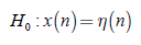
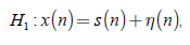
The spectrum sensing goal in cr is centered in hypothesis (Eq. (1,2)):

()1

()2

where x (n) is the signal received by the secondary user; s (n) is the signal trans mitted by the primary user; ƞ (n) is an additive white Gaussian noise (AWGN); and H ₀ is the null hypothesis that indicates absence of licensed user signal.

1.2 Energy Detection (ed)

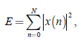
In the ED technique, the signal power is measured in a particular frequency band along the time axis. The decision parameter for edis shown in Eq. (3):

()3

where N is the number of samples in the analysis window. In this case, given a threshold ϒ, if E>ϒ, the hypothesis H ₁ is accepted, and if E < ϒ the hypothesis H ₀ is accepted.

1.3 Cyclostationary Detection (cd)

The cyclostationary features are produced by the signal periodicity (or by the periodic ity of its statistic measures). The cyclic spectral analysis implies second order trans formations of a function and its respective spectral representation ⁸. The distinction between primary and secondary users is possible only if different cyclic frequencies are involved ⁹.

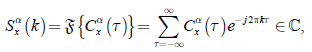
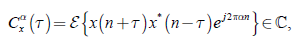
The Spectral Correlation Density (scd) of a signal could be calculated by Eq. (4) (10):

()4

whereis the Fourier Transform; α is the cyclic frequency andis the Cyclic Autocorrelation Function (CAF) of x, defined in Eq. (5):

()5

where x ^* is the conjugate version of x. The caf exhibits peaks when the cyclic frequency _ has the same value of the fundamental f requencies of the t ransmitted signal ⁶.

The frequency-smoothing method is used to estimate the scd as recommended in ¹¹

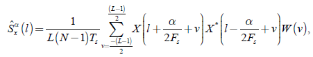()6

Where:

()7

where N is the number of samples in the analysis window; s T is the time-sampling increment; s F is the frequency-sampling increment; and () Wvis the frequency smooth ing function centered at 0 =vof width L.

2. PROPOSED SCHEME

2.1 Blind Source Separation

Blind source separation techniques allow separating different signals without previous knowledge about the signal features. The most common technique for source separa tion is ica.

In ica, the received signal is assumed as a linear mixture of statistically indepen dent sources that could be separated maximizing the non-Gaussianity. This technique requires a mimo system with p sources and m receptors (p ≤ m), their combined out puts build the matrix of observable data 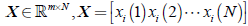, where xi (j) is the j-th sample (or time instant) of the signal in the i-th receptor, and N is the number of samples in the analysis window. The principal idea in ica, is to get the original sources S from the matrix of observable data X as in Eq. (8):

()8

where is the mixture matrix and 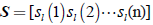, where is the j-th sample (or time instant) of the signal transmitted by the l-th source, and N is the number of samples in the analysis window.

If the matrix A is known, the source data could be reconstructed by its pseudo-inverse matrix. If A is unknown, it is necessary to calculate A and 𝑺 from the obser vation matrix X as in Eq: (9), in such a way that the estimated components ŝ must be the linear combination of the data with the maximum independence ¹².

()9

where is a matrix that maximizes the statistical independence.

2.2 ms - ica

In this work, the algorithm proposed by Molgedey (¹³), ms - ica, is chosen (Algorithm 1 (14)) due to its performance in online applications (¹⁵).

Algorithm 1. ms - ica

Input: Data matrix X

Output: Estimated source matrix Ŝ

1. Center the observation matrix variance 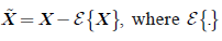is the expectation operator.

2. Whitening: transform X with non correlated components and unit variance

a) Calculate the covariance matrix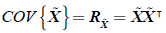

b) Find the eigenvalues where V is the eigenvector matrix and Ó is a diagonal matrix of eigenvalues

c) Find the transformation matrix

d) Calculate the data matrix projection

3. Fix the lag τ

4. Solve the eigenvalue problem for the ratio matrix is the autocorrelation matrix of S at lag τ

5. Compute the matrix A as the eigenvalues matrix of Q (16).

6. Find the mixture matrix W = A ^-1

7. Calculate the source matrix ŝ by Eq. (9)

The lag parameter τ could be calculated as proposed in ¹⁶: a) compute ŝ as in algorithm 1 for τ =1; b) find the minimum value of δ (τ ) in Eq. (10) by iterating the parameter τ, where ^_cs are the normalized autocorrelation functions; and c) recalculate ŝ after q iterations.

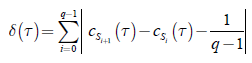()10

2.3 Single-to-Multichannel Conversion

Aiming to find a matrix representation for a single-channel data, the procedure pro posed by (17) through ssa was applied as follows:

1. Calculate the autocorrelation function of x (n) as in Eq. (11), where l = 0,…,1 =…L− and L is the analysis window length. A suitable value for L is an important issue in ssa. In this work, the value is fixed as one more than the number of peaks in the periodogram of the received signal x (n), aiming to find an approximate number of expected sources.

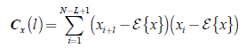()11

2. Find the Toeplitz matrix ^_To of the autocorrelation function.

3. Calculate de eigendecomposition of ^_To as ^_To = V Ó _^VT . Sort eigenvalues (Ó) in descending order and preserve the most informative components.

4. Create the Hankel matrix TH of x (n), with K = N −1 + L (Eq. 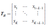(12)).

()12

5. Project H T into the subspace of eigenvectors of 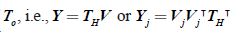The main idea is to define the temporal behaviors.

6. Reconstruct X as a sum of the projections obtained by the inverse Hankel procedure of Y j .

7. Calculate algorithm 1 with the following modifications:

a. Choose two subsets, i.e., j = 2.

b. Use the first subset as the input of the algorithm.

c. Divide the remaining subset into two subsets.

d. Go to step b. and repeat the process.

3. EXPERIMENTAL SET-UP

The different schemes for spectrum sensing are tested with an artificial mixture signal defined by Eq. 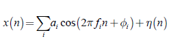(13).

()13

The length N of x (n) with n =1,…,N is fixed in 4,000 bins, the sampling frequency ^_fs = 10 kHz, and the parameter L= 512 for the cyclostationary analysis (smoothed window length). The white Gaussian noise ƞ(n) is a variable parameter, with SNR between 10 −and 20 dB.

In order to check the technique’s efficiency, some variations in the number of original sources and noise power ( ^_Pƞ ) are made. The amplitude of the sources is ai = 1 and the phase Φi =0 . For ED, a system with six fir filters is implemented, each one with order 100, Hamming window, bandwidth 520Hz, a center frequency of ^_fi and 10Hz of overlapping; then, the procedure recommended by (18) is followed for each channel with 1,000 Monte Carlo simulations, aiming to determine whether a channel is available or not. For CD, the parameter μ is fixed by heuristic tuning and it determines when a peak of the caf corresponds to a fundamental frequency or not.

The elapsed time that the algorithms took to run is measured in an Intel ^® Core™ i5-2,400 with 4 GB of ram memory and Python ^® of 64 bits.

4. RESULTS AND DISCUSSION

Table 1 summarizes the results for the three tested schemes. The technique most sensi tive to noise is ed, with the disadvantage that if the frequency bands are unknown, the algorithm is unable of detect different frequency components. The mean time elapsed for this technique is 97.85 ± 1.02 s, and tends to increase with the number of channels. The cd and ms-ica’s are noise-robust algorithms. The time elapsed for cd is around 106.94 ± 1.77s that could be compensated by its precision. The cd sensing technique generates some false positives, but the rate of false negatives is zero. If the intention of the secondary user is to search for vacancy without disturbing the primary user, and the time is not a critical issue in the application, this technique could be a convenient solution. The only inconvenient detected is the parameter μ, because the algorithm performance depends on the choice of this parameter.

Table 1 Spectrumsensing test results 

Source: authors

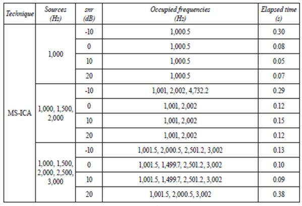
The proposed ms-ica technique exhibits a suitable compromise between time and performance. The algorithm is fast enough to sense without causing long interrup tions in transmissions. The major disadvantage is the misdetection of some sources. To overcome this inconvenient, it is recommended to run the algorithm a couple of times and increase the amount of information about the frequency occupancy. The remarkable aspect is the elapsed time (0.15 ± 0.1 s), especially for online applications with demanding time issues.

5. CONCLUSION

A technique for spectrum sensing based on blind source separation is explored. The methodology includes a single-to-multichannel procedure through singular spectrum analysis (ssa), aiming to simulate a mimo communication system. In this work, three approaches were tested: Energy Detection, Cyclostationary Analysis and the proposed scheme with ms-ica. The methodology is proved on a collection of artificial mixture signals with different frequencies and noise power. The proposed scheme is able to detect most of the sources, even with high noise presence, with low time consumption. The most accurate technique is Cyclostationary Analysis but it is more demanding in terms of time than the others. As future work, it would be interesting to deal with other kinds of modulations, codifications and channel models.

6. ACKNOWLEDGMENTS

Thisworkissupportedby “Validación de algoritmos de aprendizaje automático usados en sistemas de telecomunicaciones de radio cognitiva (Código No. 737)” financedby Universidad de Medellín and by “Ayudas para la realización del doctorado” (RR01/2011) of the Universidad Politécnica de Madrid y TEC2012-38630-C04-01 del Ministerio de Educación de España”