1. INTRODUCTION

Ultrasonic elastography (USE) is an imaging technique that allows calculating the degree of hardness of materials from ultrasound (US) echoes reflected on a material. It has become a promising technique to determine the degree of tissue elasticity from its compression, allowing distinguishing a healthy tissue from one with abnormalities, being very useful in the improvement of medical diagnosis of diseases affecting the biological tissues, including cancer. In the literature, ultrasound elastography has been used as a diagnostic tool for breast cancer ^1-2, thyroid cancer ³, prostate cancer ⁴, carotid plaque elasticity ⁵, liver fibrosis ⁶, among other pathologies.

Static USE introduced in ⁷ is a technique where an external quasi-static compression is axially applied to the tissue to acquire successive RF frames. The RF data sequence is processed to obtain the images before and after compression. Typically, a block searching algorithm finds the axial and lateral relative displacements between these two images. The axial strains field is calculated as the gradient of the axial displacements.

The previous work in ⁸ has shown how the quality of the elastogram (the image with elasticity information obtained by the elastography technique), depends on several factors such as non-uniform compression, out-of-plane motion, strain-dependence of noise in elastograms frequency-dependent attenuation, uncontrolled and unwanted transducer motion introduced by the operator, the used displacement computing algorithms, among others. Therefore, one of the main drawbacks of this procedure in clinical practice concerns to reliability of the diagnostics derived from an elastogram. The works in ^9-11 evaluate the performance of USE in the diagnosis of breast lesions, concluding that at present, elastography does not have the potential to replace conventional B-mode US in the detection of breast cancer. However, improvements such as the achievement of quantitative measurements could enhance its clinical acceptance.

This work addresses some needed procedures and algorithms in order to obtain an ultrasound elastogram, and discuss the difficulties to be overcome to achieve clinical diagnosis of diseases using USE. This paper has been organized as follows: Section 2 presents the computing algorithms and procedures to obtain a normalized elastogram. Section 3 presents validating results of the procedure to get the elastogram with some discussion about the difficulties to be overcome in order to achieve confident clinical diagnostics from USE. Finally, Section 4 presents some conclusions and suggestions for further work.

2. METHODS

In this work, a set of software functions for OpenCv and Matlab(r) has been built, which allows the obtaining of a normalized elastogram useful for elasticity analysis. The processing procedure can be summarized as follows: (I) raw RF of pre and post-compression frames are used to compute the relative axial and lateral displacements between this pair of frames; (II) a spatial gradient applied to the axial displacements image is used to compute the strains image or elastogram; (III) a normalization procedure is applied to the strains image in order to compensate the depth dependency of the strains or elevation of the probe during the scan; (IV) using the RF echoes from websites for both, phantom and patients diagnosed with some diseases, a discussion is made about difficulties and requirements to achieve confident and conclusive clinical diagnostics of diseases using USE.

The following subsections describe the theoretical foundations and the algorithms used in this work through these five stages of processing.

2.1 Axial and lateral displacements

This paper focuses on the free-hand quasistatic axial strain imaging technique, which has shown to be very promising in clinical trials and has been commercialized by several manufacturers ^12-13. The clinician holds an ultrasound transducer over the area of interest while gently varies the contact pressure, thus inducing mechanical stress in the targeted tissue, predominantly in the axial direction. Consecutive frames in the RF data sequence are compared conforming a set of reference images (before the compression), and deformation images (after static compression) to estimate the resulting axial and lateral displacements. Most of the useful elasticity findings from an elastogram can be obtained from the axial displacements, even though lateral displacements can be used to get more accurate results in some specific cases ^14-15.

Numerous algorithms have been reported in the literature aimed to the displacements computing, being the key differential subjects: speed, accuracy and robustness. The work in ⁸, made a comparison about the impact on the quality of the elastogram, of the algorithms used for the displacements calculation. For a better understanding of the procedures and algorithms, excerpts from this work have been replicated in this paper.

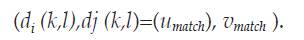
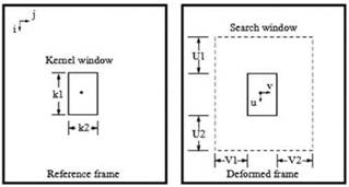
Algorithms for displacements computing can be roughly classified as block matching based or not block matching based. Consider figure 1, where a kernel centered at location (i, j) in the reference frame must be matched with a kernel of the same size in the deformed frame, whose center should be displaced due to the exerted compression. The kernel is then swept through the whole reference frame and for each center (i, j), a search window greater than the kernel and centered at the same location, is settled into the deformed frame. The displacement of the center of the matching kernel is established in the relative coordinates of a search window (range of kernel centers) defined by -U ₁<u<U₂ and -V₁< v <V₂, where U ₁, U₂, V₁ and V₂ are the lengths of the search window in up, down, left and right directions, respectively. The height and width of the search region are U= U ₁+U₂+1 and V=V₁+V₂+1 respectively. The relative locations of the centers of the matching kernels (U _match,V_match) are stored in the axial displacements image d _i and lateral displacements image d _j as:

The distribution of the displacements are usually not as fine as the RF samples, i.e. if i axis is swept in k steps and j axis is swept in l steps, the resulting displacements are sub-sampled images of the original frames.

Figure 1 Definition of kernel and searching region. 

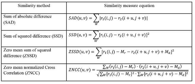
Typical implementations of the matching blocks algorithms need a good selection of Uand V, which must be large enough to ensure that the displaced kernel can be contained in the search region, thus avoiding high decorrelation of the resulting matching blocks. About how to decide which kernel in the deformed frame matches to the kernel in the reference frame, the decision is made from the minimization or maximization of a similarity measure. Numerous similarity measures have been proposed in the literature to this end, which have been used in the computer vision field since long time ago. Some of them are summarized in the table 1, where W is the kernel window centered at (i,j), r₁ and r ₂ are the pre and post deformation RF frames, u and v are the relative axial and lateral displacements of the kernel in the deformed frame, and M r and M d are the means of the kernel window over the pre-deformed and post- deformed frames respectively. Thus, for each pair (i,j) on the pre-deformed frame, the corresponding relative displacements of the post-deformation frame will be those pair (u,v) maximizing (ZNCC) or minimizing (SAD, SSD, ZSSD) the similarity measurement criteria on the whole searching region.

The basic exhaustive matching blocks algorithm can be improved with multilevel searching strategies which can be faster due to a progressive refinement of the precision at different levels of processing. They can automatically compute convenient kernel windows to avoid high decorrelation of the matching blocks. One example of this approach is the hybrid method ¹⁶ of estimation of displacements which has three processing levels.

Table 1 Some similarity measurements used for matching of blocks methods. 

The main drawback of the optimization process for block matching in the previous methods is time consumption. In the Dynamic Programming Approach (DPA), a cost function C is globally optimized in a non iterative way through recursive computing. In this way, time consumption is drastically reduced and the cost function can be used efficiently to penalize non smooth adjacent displacements, preventing noisy effect on decorrelated data. This method can be referred as a non-matching blocks method since its matching process is achieved as a whole optimization process of the cost function at sampled data level. Details of this technique can be consulted in [¹⁷].

2.1 Axial strains

Consider image's variation before and after deformation described in figure 2, where an affine transformation can be established in order to describe the deformation of the image based on its axial and lateral displacements. Q(x,y) is an arbitrary point in the pre-deformation sub-image and its corresponding point in the post deformation sub-image is Q'(x,y'), where the points Q and Q' have been matched through registration. Taylor expansion for point Q'(x' ,y') is made and the high order infinitesimal term is omitted. Then the relationship between Q'(x' ,y') and Q(x,y) can be gotten as follows:

Figure 2 Sketch for affine transformation of an image. Source ¹⁸  

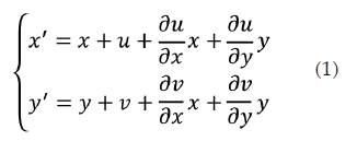
In (equation 1), the first order partial differentials denote the strain profiles. Note that for the case of a rigid body, the difference between the images before and after deformation corresponds just to a displacement, not to a deformation, and strains would be zero. Therefore, higher strains values correspond to softer materials while low strains values correspond to harder materials. The strains ∂u ∂x and 𝜕𝑦 𝜕𝑥 are referred as normal strains (axial and lateral respectively), and they are related with amount of stretch or compression along material line elements or fibers. The normal strain is positive if the material fibers are stretched and negative if they are compressed.

The strain map is usually displayed as a grey level image and is known as elastogram, being an indicator of the relative elasticity properties of the materials in the RF ultrasound frames. Even though both, axial and lateral normal strains have been reported as containing useful information for clinical diagnostics, the axial strain usually is the only one used for elastography. The algorithms used to calculate this map consist of calculating the spatial gradient of the axial displacements. Many filters used in computer vision are available to this end, and since the gradient is a noisy operation, some kind of smoothing filter, such as the Kalman filter ¹⁴, is necessary to improve the appearance of the image.

2.3 Strains normalization

The quality of an elastogram can be estimated from its signal to noise ratio (SNR) map, which is defined in elastography as SNR _W = s /a ¹⁷, where s and o are the spatial average and variance of a window W on the strain image, respectively. The strain map is computed moving the analysis window trough the whole image. High SNR values indicate uniformity of the strains in regions of similar elastic properties, which in some sense indicate a certain confidence grade of the computed mean strain.

Axial relative displacements have not a uniform distribution through the whole echo frame. This makes sense since the regions near the ultrasound probe, where the compression is done, experience big axial displacements, in contrast with the low displacements registered in deeper regions, far from the compression area. This fact is transferred to the strain map and contributes to low SNR of the elastogram, besides to making the elasticity reading difficult, given that it turns out to be dependent on the depth in the RF frame.

To compensate for this effect, several authors referred a normalization procedure, which in fact is a depth dependent compensation procedure. In ¹⁹, for example, the basic problem of finding an appropriate strain scale for each image can be solved robustly by fitting a plane to the entire set of displacement estimates, {d(x,y)}. This is performed in that work through the method of precision-weighted least squares, thereby determining an "normalization" strain. One possible equation of the fitted plane can be as follows:

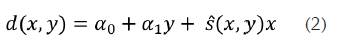
Where s (x,y) is a normalization strain which is computed as follows:

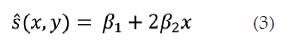
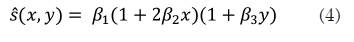
(Equation 3) can adjust for the reduced stress at greater depths away from the probe, as the stress spreads out into the surrounding tissue. Another option for a normalization strain is adjusting for the possibility that the probe may rotate about the elevational axis during the scan, resulting in stress variation over the lateral direction. (Equation 4) is appropriate to this end.

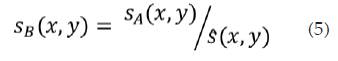
The strain estimates should be scaled so that the dynamic range in the display is from zero up to a fixed multiple of the normalized strain, s. Denoting prenormalization strain estimates and post-normalization strain by s_A and s_B respectively, then:

3. RESULTS

In this section, the aforementioned procedure has been applied to pre-compression and post-compression echo data for three study cases considered: (I) a phantom described in ¹⁴ and ¹⁷ whose RF frames are available from the AM2D software at the website in ²⁰; (II) RF frames collected for two patients with a linear transducer array from the Antares(tm) System, available at the Insana Lab web site in ²⁰, corresponding to a benign fribroadenoma and an invasive ductal carcinoma diagnostics. For the three study cases, the probe is manually pressed into the surface scanning in the anterior-posterior direction during some time period. Just two RF frames have been considered for each case in this study, one at the beginning of the echoes collection, and the other one, once the compression has been settled. The axial displacements have been computed using the AM2D ²⁰ MatLab(r) functions which implements the DPA algorithms proposed in ¹⁴.

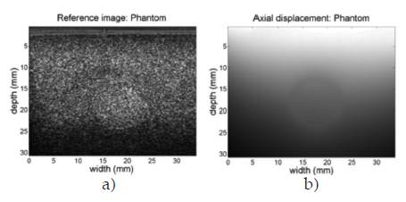
For analysis purposes, initially consider the phantom case analyzed in ⁸. Figure 3 shows the B-mode pre compressed frame (reference frame) and the computed axial displacements, where the top to bottom in the figure is the axial direction and the region at top is the closest to the ultrasound probe, and the region at bottom is the deeper region reached by the echoes.

Figure 3 a) Reference image: Phantom. b) Axial displacements: Phantom. 

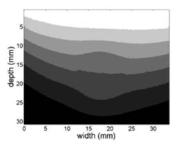
As has been reported in literature, axial displacements are dependent of the depth in the image. For a better understanding of this phenomenon, a k-means segmentation procedure was computed in order to reveal groups of similar displacements on the axial displacements graph. The result of this procedure for seven groups is shown in figure 4. The grouping of regions with similar axial displacements reveals a clear dependence between the depth and the values of the displacement, as intuitively is expected since the regions near the surface compression should suffer greater displacement than those who are distant to the probe.

Figure 4 K-means segmentation of axial displacements. 

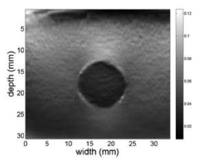
Using the spatial gradient plus a Kalman filter designed in ²⁰, the axial strain elastogram for the phantom case is shown in figure 5. The color map in figure must be interpreted as follows. Colors towards black in the map correspond to regions experiencing lower relative deformations, i.e. regions of increased hardness, while colors towards white in the map correspond to regions experiencing higher relative deformations, i.e. softer regions. The depth dependence in the axial displacement map is also translated to the computed axial strain, since the spatial gradient of the axial displacement keeps this multiplicative factor.

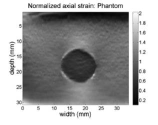
(Equations 4 and ⁵) were used to obtain the normalized axial strain of figure 6. Note that this normalization procedure achieves a correction of the strain information at deeper regions on the axial direction, which permits having a right hardness indication of the materials in the phantom since this phantom consists of a set of inclusions in a gelatin, where there is a hardness region of disk shape in the middle. The results of the elastogram suggest that the disk is three times harder than the environment, which is consistent with the known physical phantom data.

Figure 5 Axial strain elastogram: phantom. 

Figure 6 Normalized axial strain elastogram: phantom. 

The normalization process enhances the SNR too. Figure 7 shows the SNR images resulting from sweeping the elastrogram of the phantom with a square window of size 7x7 pixels and mapping the SNR values over a gray color map, where black regions represent poor uniformity of the predicted elasticity whereas white regions represent high uniformity of the predicted elasticity. Fig. 7 (a) is the SNR of the elastogram without normalization, while Fig. 7 (b) is the SNR image of the normalized elastogram. The circled shape of the black regions agrees with the border of the disc in the phantom, where elasticity changes are expected. The normalization procedure was able to increase the mean SNR value from 10.27 dB to 11.18 dB in this study case.

The elastograms of patients present challenging problems due to the impedance changes suffered by the echoes through the various kinds of tissues, blood vessels, changes in elevation of the ultrasound probe, etc., which results in increased noise levels. The results are highly dependent of the size of the searching region for the axial displacement. Thus, higher sizes of searching windows allow the finding of suspecting masses in the frame, but resolution of the information is decreased. Lower sizes of searching windows result in noisy elastograms. In this work, axial size of the searching window has 100 pixels long, while lateral size of the searching window has 6 pixels long, allowing the detection of masses of approximately equal area.

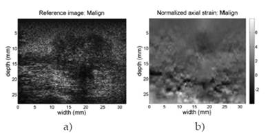
Figure 8 shows the B-mode reference image and the normalized elastogram for the patient diagnosed with benign fibroadenoma (breast). Colors in the map reveal that tissues on the image have relatively the same low hardness, allowing discarding the masses in the reference image as having a malign classification. Figure 9 shows the same images for the patient case diagnosed with ductal carcinoma (breast). The hard black color inside the defined closed region at the top center of the image reveals the presence of a hard mass in that region. Full colored elastograms facilitate the interpretation, but there is need for automatic algorithms able to classify the tissues as benign or malign, since there is no way to establish a reference of hardness over the image.

Figure 7 a) SNR without normalization b) SNR with normalization. 

Figure 8 a) Reference image: Benign b) Normalized axial strain: Benign. 

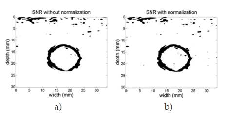
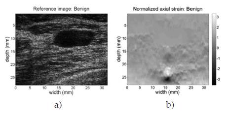
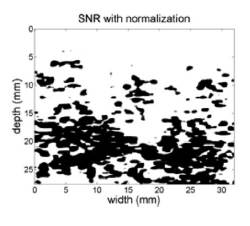
Figure 10 shows the SNR of the normalized elastogram of the malign study case. This figure confirms the difficulties to build automated algorithms to establish benignity or malignity of masses found in the US echoes, due to the existence of non confident regions distributed through the whole elastogram.

Figure 9 a) Reference image: Malign b) Normalized axial strain: Malign. 

Figure 10 SNR with normalization: Malign. 

A brief discussion about the obtained results, summarizing troubles and prospects for clinical diagnosis of the explored technique is needed. Elastography has been reported since about 1990 as a promissory technique useful for clinical diagnostic of diseases such as several kinds of cancer. This work has explored reported techniques and algorithms which led to obtain the relative hardness of the materials from ultrasound echoes. The previous work in ⁸ shows how similar results can be obtained from different displacements algorithms, differing principally in computational efficiency issues. However, clinical studies about the confidence of these diagnostics reveal several difficulties to be overcome in order to make those promissory benefits, a reality. In this work, regardless of the mechanical and technical difficulties for the free hand technique to obtain repeatable results, many troubles related to the elastogram interpretation have been identified when these methods are applied to echoes from biologic tissues. They can be summarized as: (I) the elastogram is highly dependent on the parameters of the algorithms used to computing the axial displacements, so the clinical experience of an ultrasound technician is necessary in order to obtain reliable elastograms (II) masses on the US echoes have not clearly defined boundaries, thus hindering both, manual identification as automatic regions of interest, (III) the SNR of the elastograms is not uniform, which affects the reliability of results in all regions of the image. In current practices, the elastography images are presented side by side with 2D US B-mode image. The user needs to manually identify the probable lesions and draw corresponding boundaries around the lesions, and then the system displays the measured area and ratio of areas of strain elastography image besides the US B-mode images. The main drawback is that the user (physician or radiologist) is expected to draw the boundary across the probable lesions which are not very accurate. This manual boundary delineation makes the process subjective, and highly dependent upon the user's expertise. However, computational intelligence tools arise as a possible solution to the problem of how to achieve reliable clinical diagnostics, since the ultrasound technicians' expertise can be used to both, to configure the parameters of the algorithms and to establish a reliable clinical diagnosis.

4. CONCLUSIONS

The USE has been reported as a promissory technique for medical diagnostics for nearly twenty years, with numerous commercial devices currently available. These devices are so expensive and not available to the majority of potential users in developing countries. Medical acceptance of these diagnostics remains at low levels due to both technical and computational difficulties in order to obtain reliable and conclusive results. However, nowadays it is possible, with not expensive electronic cards and better computational algorithms, to contribute to improved diagnostic procedures in medicine.

In this work, a procedure to obtain elastograms has been presented and verified. Further work will be addressed towards procedures to achieve reliable and automatic diagnostics, and towards the construction of low cost devices to these end.

ACKNOWLEDGEMENT

The authors wish to thank to the University of Cauca in Colombia for supporting this research.