


Services on Demand
Journal
Article
 English (pdf)
 Article in xml format
 Article references
 Send this article by e-mail
Indicators
-
 Cited by SciELO
 -
 Access statistics
Related links
-
 Cited by Google
 -
 Similars in
SciELO
Similars in
SciELO -
 Similars in Google
Share

 Permalink
Revista EIA
Print version ISSN 1794-1237On-line version ISSN 2463-0950
Rev.EIA.Esc.Ing.Antioq no.16 Envigado July/Dec. 2011
FINANCIAL RISK ASSESSMENT OF DIFFERENT INVENTORY POLICIES
EVALUACIÓN DE RIESGO FINANCIERO PARA DIFERENTES POLÍTICAS DE INVENTARIO
AVALIAÇÃO DE RISCO FINANCEIRO PARA DIFERENTES POLÍTICAS DE ESTOQUE
Héctor Hernán Toro*, Leonardo Rivera**, Diego Fernando Manotas***
*Ingeniero Industrial y Magíster en Ingeniería Industrial, Universidad del Valle. Profesor Auxiliar, Escuela de Ingeniería Industrial y Estadística, Universidad del Valle, Cali, Colombia. htorodi@clemson.edu
**Ingeniero Industrial, Universidad del Valle; Ph.D. in Industrial and Systems Engineering, Virginia Polytechnic Institute and State University. Jefe de Departamento de Ingeniería Industrial, Universidad Icesi. Cali, Colombia. leonardo@icesi.edu.co
***Ingeniero Industrial, Universidad del Valle; Magíster en Gestión Financiera, Universidad de Chile. Profesor Asociado, Escuela de Ingeniería Industrial y Estadística, Universidad del Valle. Cali, Colombia. diego.manotas@correounivalle.edu.co
Artículo recibido 2-V-2011. Aprobado 21-IX-2011
Discusión abierta hasta junio de 2012
ABSTRACT
This work addresses the valuation of economic effects of different inventory holding policies. We study the VaR over the value of a company and the variations induced on this indicator by the changes made to the working capital, related to inventory policies. Three typical different inventory systems are studied and comparisons are drawn between different policies. Policies derived from net present value (NPV) maximization are contrasted against cost minimization, as well as against arbitrary inventory policies derived from market conditions. Every inventory system under study is evaluated using two performance indicators: NPV and VaR over NPV. The inventory policies are derived in a deterministic scenario, but are tested under the risk conditions that the inventory systems have to face. This is done by using Monte Carlo simulation. In all three of the inventory systems under study, the difference between price and variable cost is what causes the greatest variation on the NPV indicator. An important result of this work is that for the cases studied, which are rather common in the real world, the optimal inventory policies obtained by using the cost minimization approach are equally good from a risk minimization perspective than those obtained by using the profit maximization approach.
KEY WORDS: investment analysis; inventory management; Monte Carlo simulation; Value at Risk.
RESUMEN
Este trabajo se concentra en la evaluación de los efectos económicos asociados a diferentes políticas de inventario. Se estudia el valor en riesgo del valor de una compañía, además de las variaciones inducidas por los cambios en el capital de trabajo asociados a diferentes políticas de inventario. Se estudian tres sistemas de inventario y se comparan diferentes políticas. Se contrastan las políticas derivadas de la maximización del valor presente neto (VPN) contra la minimización de costos y contra políticas de inventario arbitrarias derivadas de las condiciones de mercado. Para cada sistema de inventario se estiman dos indicadores de desempeño: VPN y VaR del VPN. Las políticas de inventario se construyeron en un escenario de certeza, pero se evalúan incorporando diferentes condiciones de riesgo, para lo cual se utiliza simulación de Monte Carlo. Las conclusiones se obtienen a partir del desempeño observado en diferentes casos de estudio, usando ambos indicadores. En los tres sistemas de inventario bajo estudio, la diferencia entre precio y costo variable es lo que causa la mayor variación en el indicador del VPN. Un resultado importante de este trabajo es que para los casos estudiados, más bien comunes en el mundo real, las políticas de inventario óptimo obtenidas por minimización de costos son, desde la perspectiva de la minimización de riesgo, tan buenas como las obtenidas mediante maximización del beneficio.
PALABRAS CLAVE: análisis de inversiones; administración de inventarios; simulación de Monte Carlo; valor en riesgo.
RESUMO
Este trabalho concentra-se na avaliação dos efeitos económicos associados a diferentes políticas de estoque. Estuda-se o valor em risco do valor de uma companhia, além das variações induzidas pelas mudanças no capital de trabalho associadas a diferentes políticas de estoque. Estudam-se três sistemas de estoque e comparam-se diferentes políticas. Contrastam-se as políticas derivadas da maximização do valor presente neto (VPN) contra a minimização de custos e contra políticas de estoque arbitrárias derivadas das condições de mercado. Para cada sistema de estoqueestimam-se dois indicadores de desempenho: VPN e VaR do VPN. As políticas de estoque construíram-se em um cenário de certeza, mas avaliam-se incorporando diferentes condições de risco, para o qual se utiliza simulação de Monte Carlo. As conclusões obtêm-se a partir do desempenho observado em diferentes casos de estudo, usando ambos indicadores. Nos três sistemas de estoque baixo estudo, a diferença entre prego e custo variável é o que causa a maior variação no indicador do VPN. Um resultado importante deste trabalho é que para os casos estudados, mais bem comuns no mundo real, as políticas de estoque ótimo obtidas por minimização de custos são, desde a perspectiva da minimização de risco, tão boas como as obtidas através da maximização do benefício.
PALAVRAS-CHAVE: análise de investimentos; administração de inventários; simulação de Monte Carlo; valor em risco.
1. INTRODUCTION
The usual approach for the economic valuation of projects begins with the creation of a cash flow, in which the analyst makes some estimation of future incomes and expenses. This makes it possible to account for net cash flows. Many of the cash flow parameters are random variables for most real projects, which turns the valuation into a complex problem. Simulation is usually applied to handle this situation, but the analysis of simulation outputs requires statistical tools and statistical indicators designed for comparisons between different alternatives and scenarios.
The Value at Risk (VaR) indicator is widely used today in financial institutions, as well as in the economic valuation of portfolios within the financial sector. VaR is a single number that measures the maximum potential loss in the present value of a portfolio, as long as the market conditions behave in the usual way (i.e., the market exhibits conditions similar to its historical behavior) (Linsmeier and Pearson, 1996). The idea of having a "portfolio" comes from the financial sector, but in a general way, it is possible to see a real project as a portfolio, in the sense that you need to make an investment to have the project in operation, and after the investment has been made, some economic returns can be expected in the future. For example, buying some treasury bills now and selling them after a while at a different price, hopefully higher.
The effort required for valuing a real project is usually higher than the required for valuing a financial portfolio, especially if the portfolio is composed of standardized financial instruments. For a real project, the analyst should understand the intrinsic nature of the business, identifying the main elements that affect the economic value of the project, model their behavior, and forecast them. Even if just a couple of alternatives that sell the same final product in the same market are being considered, modeling each of them is a different exercise. Each alternative differs in their internal processes and decisions.
2. PROBLEM PRESENTATION
Real projects, as well as financial instruments and portfolios, are affected by the uncertainty and risk observed in various factors, including markets, political environment, natural environment, just to mention a few. By uncertainty we refer to events that cannot be represented by probability distribution functions, and by risk we refer to those that can. Traditional methods for valuing a project use a static representation of critical future parameters, especially those that are outside the control of the project owner. This lack of control may considerably influence the main performance indicators. A single static forecast of critical parameters is not recommended for the valuation of real projects, since projects will face risk. The final values for parameters can be very different from the ones forecasted in a single scenario.
One approach to deal with risk has been the formulation of deterministic scenarios instead of the use of a single forecast. Scenario generation has at least two hurdles in its implementation: the identification of a set of scenarios that truly represent the future possibilities of the real world system and the assignment of a probability of occurrence to each scenario, since not all are equally likely to happen. Since the possibilities of behavior in a real system are basically endless, it is not an easy task to determine a subset of scenarios that represent future behavior. The assignment of probabilities for each scenario is also sometimes a subjective process, therefore exposed to human misperceptions.
Simulation is a practical approach to the analysis of the real system, assuming that it is possible to set up a formal representation of the system (mathematically and computationally). Simulation can be used to calculate performance indicators given a set of parameters constructed from the real world. The basic idea is to generate a large quantity of scenarios (each scenario is determined by the set of values of the parameters), to calculate the performance indicators for each resulting scenario. At the end, the analysis is focused on the different observed values for those indicators. Analysis is usually done by identifying probability distributions functions associated to the performance indicators.
Analysis of real projects under risky conditions is a topic that has been studied by academics and practitioners for some time. This paper builds upon ideas presented in previous documents related to the development of a performance indicator that deals with risk quantification, while at the same time measures how good a project is from a financial point of view (Ye and Tiong, 2000). Specifically, the problem is to quantify the financial risk of a manufacturing system that applies a given inventory holding policy. The expected result is an indicator of VaR type that will be used for selecting an inventory policy that maximizes the present value of a project, while exposing the company to an acceptable level of risk. As in previous works (see Section 3), the economic analysis is performed in a continuous time framework. The cash flow is constructed in this continuous framework, and a discount rate is used to estimate the net present value of the project over an infinite time horizon. A simulation tool is used to generate random scenarios and calculate a new estimation of the NPV for each of them. Finally, a VaR indicator over the NPV accounts for the implicit risk for the system, related with the inventory policy and the parameters of the system.
3. PRELIMINARY RESEARCH
Hadley (1964) developed a comparison between optimal order sizes for an inventory system with fixed order quantity, when those orders are derived using two approaches: the first one is the usual minimization of average long run cost and the second one is the minimization of a cost function that accounts for the time value of money, using a discount rate. Hadley proposed this methodology some forty years ago, and his conclusion was that for the inventory systems that he studied there was no difference in the order size when using any of those approaches. However, works presented after this seminal paper have shown that differences do occur, unless some assumptions can be considered. These assumptions include parameters that do not change their value for long periods and very low discount rates (usually less than 1%). None of these two conditions are observed in the industrial world today, so the conclusions suggested by Hadley are no longer applicable today.
Kim, Philippatos and Chung (1986), Roumi and Schnabel (1990), and Chung and Lin (1995) proposed a valuation of inventory decisions under a financial framework treating the inventory like any other asset of a company. The shareholders usually expect the investment in assets to be productive, generating an adequate financial return. The usual explanation for not valuing the inventory from a financial framework is that inventory decisions are usually beyond the reach of the financial manager, and production managers do not use a financial approach for making decisions. They usually use a costing approach. These works conclude that there are differences between inventory policies, specifically the order sizes, when those order sizes are derived using the NPV maximization instead of cost minimization.
Hill and Pakkala (2005) proposed a discounted cash flow approach for finding a good inventory policy in a system that uses periodic revision (every R units of time). The amount ordered each time is variable, calculated as the difference between a maximum inventory level previously determined (denoted as S) and the inventory available by the time the revision is made (this inventory policy is often referred as R,S). The authors focus their attention on the cash flow derived from applying the inventory policy, instead of just calculating the cost related to it. Demand is modeled by using a Poisson distribution. They considered a deterministic lead time and allowed backorders for unsatisfied demand. The optimal inventory policy is found using NPV (net present value) as the performance indicator.
Disney and Grubbstrom (2004) studied a manufacturing system also with an R,S inventory policy, in which the demand is modeled using a stochastic autoregressive process. The production/distribution lead time is set to one period, and the demand is forecasted using exponential smoothing. They approached the problem of determining the cost performance of an inventory holding policy including new cost elements, in particular, the cost of requiring additional production capacity, as well as the cost of having extra production capacity. Those two cost elements are not considered as necessarily symmetric. Every cost element is modeled using the lineal form of the functions. Their main conclusion is that optimal policies coming from the usual cost approach are not necessarily optimal in the presence of new cost elements. Also, they have found that if one considers the cost of the bullwhip effect as a part of the cost of applying some inventory policy, then the optimal values derived from the usual cost minimization approach are also invalid.
Bulinskaya (2003) introduces the analysis of inventory management in the framework of corporate risk management. Her work starts criticizing the usual cost approach, specifically the static nature of the framework employed to calculate cost. She emphasizes that real systems are dynamic by nature. Also, previous models do not include capacity constraints, therefore assuming that it will be possible to acquire any amount of product suggested by an inventory policy, while in the practice there are budget and availability constraints. The point of view used by Bulinskaya is that the inventory is just another investment option to the decision maker, and thus, the optimum inventory policy can be determined by solving an investment selection problem that can include other possibilities (assets) besides the inventory. The author uses the approximation of Cox-Ross-Rubinstein (1979) for modeling the financial market, and proposes some optimal strategies derived from that formulation.
Naim, Wikner and Grubbstrom (2007) studied the problem of selecting an order policy in a planning and control production system. The study is carried over using a simulation model widely used, referred as IOBPCS (inventory and order-based production control system). NPV is again the performance indicator to be optimized, but some additional cost elements are included. The concept of variance cost is introduced, defined as the cost in which a system incurs when it is not in perfect control with respect to some previously defined goals. Two kinds of variance costs are considered: The cost of not being able to reach a production goal and the cost of holding more or less inventory than the expected amount. Authors used a formal representation of the IOBPCS model using differential equations and then solved it using a Laplace transformation. The performance indicator including variance cost is used in the valuation of make-to-order and make-to-stock systems, concluding that the specific cost structure of every manufacturing system is a critical factor in the selection of an optimal inventory holding policy.
Luciano, Peccati and Cifarelli (2003) explored the possibility of using VaR in the context of inventory management. They used both cost minimization and profit maximization. Ordering and holding costs are included in valuation of inventory policies. Since probabilistic parameters are allowed, the authors study the resulting probability distributions of performance indicators. Upper and lower bounds are calculated for VaR as a way to estimate its confidence level. Numerical procedures are recommended, due to the complexity related to modeling real manufacturing systems. The main conclusion is that there is a good chance for obtaining large errors if normality is assumed a priori for optimization criteria. Numerical exploration of solutions, including simulation, is highly advised.
Ahmed, Çakmak and Shapiro (2007) analyzed an extension of the classical multi-period, single-item, linear cost inventory problem where the objective function is to minimize a coherent risk measure.
Tapiero (2005) introduced the use of VaR (Value at Risk) in the optimal selection of inventory policies. The main idea is to introduce an ex-post analysis, instead of the usual ex-ante approach. The ex-post analysis is possible by measuring the deviations observed from a performance indicator related to its expected values. With respect to inventory, Tapiero argues that a manager would value differently the situation of having more inventory than the expected, than the undesirable outcome of losing demand for not having enough stock. Tapiero introduces the concept of a right decision cost, which is supposed to be the cost of taking a decision from which no future deviations occur. The VaR is then suggested for this ex-post valuation, but some difficulties appear due to the complexity of mathematical expressions, some of them without analytical solutions. The VaR is also identified as a good indicator because the parameters required for its calculations (probability and a confidence level) can be related with the technical characteristics of inventory systems. Borgonovo and Peccati (2009) also proposed a research about the quantitative implications of the risk measure choice on the optimal inventory policies. Those authors developed a method to select the most adequate risk indicator to use in the evaluation of different inventory problems.
Singh et al. (2010) developed a model based on the theory of Capital Asset Pricing Model (CAPM) with the purpose to determine the lot size and reorder points from minimizing present value of total cost subject to risk adjusted discount rate. Some other research that use financial indicators as performance measurement or optimization objectives has been done for the evaluation of projects within the manufacturing sector. For further reading please refer to Followill and Dave (1998), Grubbstrom (1999), Luciano and Peccati (1999), Van der Laan and Teunter (2001), Van der Laan (2003) and Giri and Dohi (2004).
4. PROBLEM MODELING
Following the work of Kim, Philippatos and Chung (1986), three inventory systems are studied: batch sales with finite uniform production rate; uniform demand with finite uniform production rate, and uniform demand with infinite replenishment rate and stockouts. The following notation will be used:
NPV = Net present value of the cash flows for the first operative cycle ($)
NPV(∞) = NPV over an infinite planning horizon ($)
C = Variable production/procurement cost ($/unit)
D = Demand rate (units/day)
E = Sales expenses per batch ($/batch)
I = Maximum inventory level (units)
P = Selling price ($/unit)
Q = Order quantity or batch sales volume (units)
S = Fixed ordering/setup cost ($/order)
T = Cycle time (days)
U = Production rate (units/day)
f = Out of pocket shortage cost ($/unit/day)
h = Out of pocket inventory carrying cost ($/unit/day)
k = Discount rate (cost of money) per period (% daily)
Case I: Batch sales, finite uniform production rate inventory system
A firm produces at a uniform rate and stores the products until they are shipped (sold) in batch at the end of each inventory cycle. It is assumed that there will be continuous cash outflows of production cost and an out-of-pocket inventory carrying cost that is proportional to the inventory level during each cycle. It is also assumed that there will be cash outflows of sales expenses such as shipping and packaging when the products are sold at the end of the cycle. Income from sales is received in full and in cash at the moment of the sale. The NPV for cash flows in this situation for one operation cycle is:
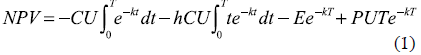
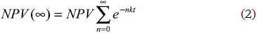
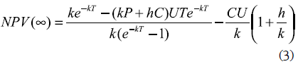
For the infinite planning horizon, the NPV will be:
The previous expression can be simplified as:
Making ∂NPV(∞)/∂T = 0 (to search for the maximum NPV value) results in:
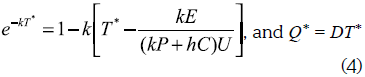
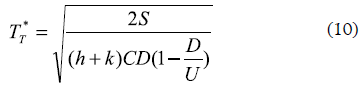
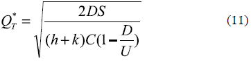
The optimal batch sales volume will be (derived from NPV maximization):
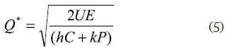
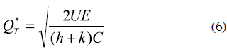
While by minimizing the cost, the optimal batch sales will be:
Case II: Uniform demand, finite uniform production rate inventory system
In this case, production and demand rate are both finite. The factory produces in lots at a uniform rate and delivers the products to a warehouse where demand happens at another uniform rate. There will be a cash outflow of setup cost at the beginning of each cycle. From time zero to τ, there will be continuous cash outflows of production cost. Throughout the cycle, there will be continuous cash outflows of inventory carrying cost and inflows of product sales. The NPV for cash flows in this situation for one operation cycle is:

For the infinite planning horizon, the NPV will be:
The optimality condition ∂NPV(∞)/∂T = 0 results in:
While by minimizing the cost, the optimal batch sales will be:
Case III: Uniform demand, infinite replenishment rate, stockouts inventory system
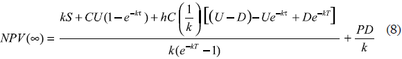
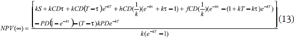
In this case, a reseller purchases products in lots for resale at the known demand rate. All demands must be satisfied, but it is allowed to be out of stock when a particular demand occurs. Demands that occur when there is a stockout are backlogged until the next procurement arrives. Backorders are met before the procurement can be used to meet any other demands. It is assumed that procurement cost for backorders will occur at the end of the cycle and outflows of ordering cost and procurement will occur at the beginning. From time zero to τ there will be continuous cash outflows of inventory carrying cost and inflows of product sales. All sells are assumed to be in cash. There will be cash outflows of backorder cost during time τ to T and a cash inflow of product sales for backordered items at the end of the cycle. The NPV for cash flows in this situation for one operation cycle is:

For the infinite planning horizon, the NPV will be:
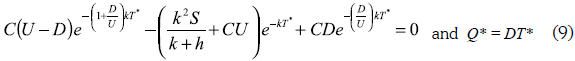
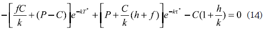
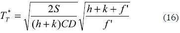
The optimality conditions ∂NPV(∞)/∂T = 0 and ∂NPV(∞)/∂τ = 0 results in

While by minimizing the cost, the optimal batch sales will be:
5. BUILDING THE VaR PERFORMANCE MEASUREMENT
The main idea is to evaluate, from a financial framework, the impact of different inventory policies over a company's value. To do so a general equation for a company's value is presented:

CV stands for company's value, estimated from the free cash flow FCF and assuming an infinite number of flows that are discounted at a rate i. The factor g is used as a decreasing or increasing rate over the FCF along the time horizon. The FCF expression is constructed adding the income I less costs of sales C and the expenses of sales management CMS. The factor I-T is related to government taxes. Depreciation and amortization are considered in the FCF taking into account that they both are non-monetary flows, and finally there are the investments in capital assets CAPEX as well as investment in working capital WK. This last term is where the inventory investments are located.
As it is clear from the CV equation, the investment related with the inventory policy has an effect over the performance measurement. At first sight, reducing the investment in WK will increase the value of CV. However, this is not always the case, especially when considering investments in inventory. The main objective of holding inventory is to anticipate demand variations, as well as changes in production conditions and lead time variability, among others. Reducing the investment in inventory can cause some demands to be not satisfied on time and hence the value of CV will decrease. Increasing inventory investment is not always a solution, because the holding cost of the inventory can be higher than the benefit of satisfying variable and uncertain demands. In this regard, finding an optimal set of operation parameters related with the inventory policy is a relevant problem for company's valuation.
In this work, the set of equations mentioned in section 4 for several inventory systems is used to build a VaR type performance indicator. For every inventory system there is an equation that measures its resulting NPV. Using a set of parameters taken from Kim, Philippatos and Chung (1986), the optimal order quantities are obtained under the two optimization perspectives: NPV maximization and cost minimization. After those optimal quantities are calculated from a deterministic point of view, their performance is evaluated under risk assumptions. In particular, for a subset of parameters (price, cost of sales, variable production cost, demand and setup/ordering cost) some probability distributions are assumed. If there were data available, the logical step would be to perform a statistical fit to a specific distribution, however, since this is not the case, a priori distributions will be used for these calculations. The benefits of using these types of distributions are documented in Johnson (1997) and Williams (1992).
By using Monte Carlo simulation multiple scenarios are generated and the NPV value is calculated for each one while the inventory policy is kept fixed using the values obtained from the deterministic scenario. Finally, the multiple results obtained for the NPV from every run of the simulation process are used to create an empirical probability distribution of the NPV. The computational software Crystal Ball automatically performs this process.
5.1 Understanding the basic idea of the VaR indicator
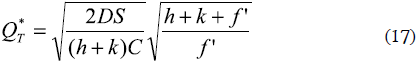
According to Jorion (1996), the VaR indicator makes an effort to consolidate the total risk exposures faced by a financial portfolio into a single number.
The VaR calculates the maximum expected loss, or equivalently, the worst scenario for the portfolio's value, given a certain probability and a period of time. Generally speaking, if the planning horizon is N periods and a % is the confidence level, then the VaR indicator can be obtained as the loss for the (100-α) percentile in the left tail, given the probability distribution for the changes in portfolio valuation for the next N periods. VaR can be seen as the answer for a single question: How bad can things go? It is measured in currency units so it is easy to understand. Additional details on several methods to calculate the VaR can be reviewed in Pritsker (1996). Figure 1 illustrates the VaR concept in a graphical way. The shadowed area below the curve denotes the probability a %, while the NPVα value corresponds to the VaR, worte scenario expected over the NPV indicator given the confidence level.
6. CALCULATING AND INTERPRETING THE VaR INDICATOR
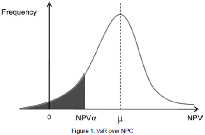
For every one of the three inventory systems described and modeled, the first step is to calculate the optimal order size under the assumption of some values for the parameters required. In the tables 1, 2 and 3 the following set of values are used (Kim, Philippatos and Chung, 1986): U = 1, k = 0.0005 (20% a year), h = 0.0005 and D = 1. The price is expressed as a function of variable cost.
In table 1, for every combination of the parameters E, C and P, the first line shows the order size derived from cost minimization perspective (hence, it is a constant number, because price variation does not affect it) and the second line shows the order size derived from NPV maximization. For those cases where there is an order size equal to zero it is because the NPV obtained is a negative value. It is possible to see that the difference between the order sizes derived from NPV and cost minimization is higher when the difference between price and variable cost increases.
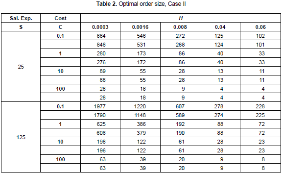
In table 2, for every combination of the parameters S, C and h, again the first line shows the order size derived from cost minimization perspective and the second line shows the order size derived from NPV maximization. It is possible to see that the difference between the orders size derived from NPV and cost minimization is lower than in the previous case. This can be explained because the process of demand occurrence is independent from the inventory policy.
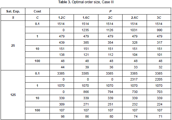
In table 3, the value for parameter f is 0.0003. For every combination of the parameters S, C and P, once again the first line shows the order size derived from cost minimization perspective and the second line shows the order size derived from NPV maximization. It is possible to see, as in the case I, that the difference between the orders size derived from NPV and cost minimization is higher when higher is the difference between price and variable cost.
In all the above three cases the order size has been obtained for a deterministic scenario. In contrast, every inventory system will have to face the variability of critical parameters. To represent this situation, the next step is to include uncertainty by allowing a subset of parameters to behave in a probabilistic way. In particular, the following subset of parameters will be modeled as random variables: price, sales expenses, variable production cost, demand, and setup/order cost. Demand is modeled as a normally distributed random variable, with mean 1 and variation coefficient 0.1. Sales expenses are modeled with a triangular distribution with parameters lower limit 23, most likely 25 and upper limit 29. Price is modeled by a uniform distribution with parameters low limit 20 and upper limit 30. Finally, the variable production cost is modeled by a normal distribution with mean value 10, and variation coefficient 0.1. It is assumed that there is no correlation between the random variables.
For the first case and the set of parameters mentioned (the mean value for the random variables), the optimal order sizes will be 71 and 53 units (see table 1), depending whether NPV maximization or cost minimization is used as optimization criteria. The order size derived from NPV maximization is higher than the other, derived from cost minimization, by approximately 34%. Given this difference in the order size, it was expected that the NPV would present a different behavior under the application of the two inventory policies. The results obtained for the NPV indicator in this case are shown in the graphics of figures 2, 3 and 4.
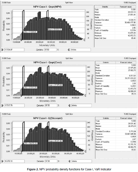
In the graphics, the NPV has been calculated under three inventory policies (order sizes). The first one is NPV maximization; the second one, cost minimization and the last one is an arbitrary policy in which the order size is four times the order calculated under NPV maximization. This last policy represents a case in which the company purchases more than the regular order size to take advantage of market discounts. For the particular case the discount has been assumed as 8% over the variable cost and it is applied to all units. The confidence level has been arbitrarily selected to be 97.5% (the usual confidence level used in hypothesis testing, for example, is 95%). Five thousand trials have been used in every case after checking that the coefficient of variability does not change by increasing the number of runs (stability of the response). Furthermore, running 5.000 trials only takes a couple of minutes of computation time.
From the graphics and the statistical information, it is possible to realize that the mean value of the NPV is similar in the three cases studied. In fact, the difference between the mean NPV for the two first scenarios (NPV maximization or cost minimization) is as much as 0.2%. The third scenario shows a variation of approximately 5% when compared against the first one. This is interesting because the variation in mean NPV is just 5%, while the variation in order size is four times the original value. Hence, the three different policies are similar when they are evaluated from NPV perspective. The other concern is the risk, which in this case is measured through the VaR. For the three scenarios under consideration the resulting VaR values are 17.535, 17.518 and 16.676, respectively. In all cases the confidence level used was 97.5%. Given the interpretation of the VaR indicator as a worse case value for the NPV, then it is necessary to select the policy in which the worst scenario has the highest value, so the best policy in this context will be to use the order size derived from NPV maximization. However, it is possible to see that the VaR for the second scenario is very close to the VaR obtained in the first one. Basically, it can be said that the first and second policy present a similar behavior also when compared using the VaR indicator. The third scenario shows a VaR of 16.676, which means a variation when compared against the VaR of the first scenario of about 900 monetary units. However, instead of making the comparison directly between VaR it is better to compare the VaR indicator against the mean value of NPV, because the VaR is a value for the NPV, the value for the worst expected case given a certain probability. For the three scenarios, the ratio between VaR and its respective mean NPV is about 62.5%. This consistency among the three scenarios means that, from a risk perspective, the three policies are also similar.
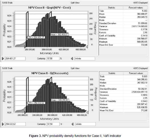
For the second inventory system, the set of parameters that are now assumed to have probabilistic behavior are: demand, normally distributed with mean 1 and variation coefficient 0.1; setup/ordering cost is assumed to have a uniform distribution, with parameters (112, 138); the price is modeled with a triangular distribution with parameters (250, 300, 330) and the variable cost is modeled by a normally distributed variable with mean value 100 and variation coefficient 0.04. k = 0.0005, h = 0.0008 and U = 5. In this case, the order size resulting from NPV maximization and cost minimization is the same quantity, 20 units. The comparison will be made against an arbitrary policy, similar to the one described before and related with market discounts. The order size is again 4 times the regular order, and the discount is again 8% applied to all units. The results are shown in the figure 3.
Figure 3 shows the results for the second case. Once again, the resulting NPV values from both inventory policies are similar, since the variation observed in NPV indicator for the two scenarios is just about 3%, as well as the VaR indicator where the variation is about 4%. The ratio between VaR and mean NPV is again consistently equal to 73%. Once again, the mean behavior of the system measured with the NPV indicator and also the risk position, measured by the VaR, are very close for the two inventory policies used, although those policies are quite different.
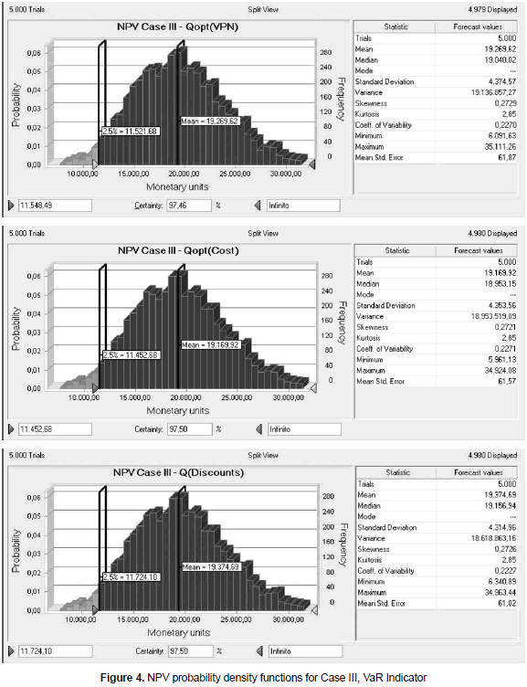
Finally, for the third inventory system the following set of parameters is used. Demand is modeled by a normal distribution with mean value 1 and variation coefficient 0.1. Setup/ordering cost is modeled with a uniform distribution with parameters (112, 138). Price is modeled with a triangular distribution with parameters (17, 20, 25). Variable cost is modeled with a normal distribution with mean value 10 and variation coefficient 0.1. Simulation outputs are shown in the graphics of figure 4.
From figure 4 and the statistical information it is possible to see that the behavior of this inventory system is quite similar to the exhibited for the two previous. Once again, three different inventory policies lead to a similar behavior in terms of mean NPV but also VaR. The ratio between mean NPV and VaR is in this case about 65%.
In all three inventory systems studied it has been identified the critical parameters that had the biggest influence on the NPV indicator. The general conclusion is that the difference between price and variable cost is what causes the greatest variation over NPV indicator. As the margin increases (price less variable cost), so does the variability over NPV, measured by its standard deviation.
7. CONCLUSIONS AND FUTURE RESEARCH
After reviewing the results that have been shown regarding the different inventory systems studied, it can be concluded that although different optimization criteria are used to make decisions about inventory policies, the system performance when applying different inventory policies is similar when it has to face the risk conditions that are inherent to its nature. The usual approach to determine inventory policies is the average long term cost minimization, approach that have been criticized because its lack of representation of the genuine conditions of the real manufacturing systems. Instead, some authors have claimed that NPV maximization should be used, since this approach is consistent with the maximization of company's value. The present work has used both approaches to derive optimal operation conditions, and in fact the inventory policies coming from every approach differ. However, when those different policies are applied to the system, and it is simulated by using Monte Carlo simulation, assuming a probabilistic behavior for a subset of critical parameters, the mean behavior observed for the system have been quite similar. In fact, from a risk perspective, it has been observed that the different policies are consistently equivalent, since for every system studied the ratio between VaR and mean NPV is a constant. From a return perspective, the analysis of the inventory systems under deterministic assumptions reveals a difference between the NPV indicators when using different inventory policies. However, the mean NPV of the system when it is calculated from the simulation process results in a very close value, especially when comparing the policies derived from NPV maximization and cost minimization. These results suggest that the usual approach used in the real world of manufacturing systems, consisting in determining inventory policies from cost minimization perspective is a robust procedure, as good as using NPV maximization, which is claimed to be more precise.
Further studies can be conducted to evaluate other inventory systems, or the same inventory systems studied in this work, but including different operation conditions, such as credit policy, for example. It is also possible to conduct studies intended to find optimal inventory policies derived from risk minimization, using the VaR indicator, or some other risk measurement.
REFERENCES
Ahmed, Shabbir; Çakmak, Ulas and Shapiro, Alexander (2007). "Coherent risk measures in inventory problems". European Journal of Operational Research, vol. 182, No. 1 (October), pp. 226-238. [ Links ]
Borgonovo, E. and Peccati, L. (2009). "Financial management in inventory problems: Risk averse vs risk neutral policies". International Journal of Production Economics, vol. 118, No. 1 (March), pp. 233-242. [ Links ]
Bulinskaya, Ekaterina V (2003). "Inventory control and investment policy". International Journal of Production Economics, vol. 81-82 (January), pp. 309-316. [ Links ]
Chung, Kun-Jen and Lin, Shy-Der (1995). "Evaluating investment in inventory policy under a net present value framework". The Engineering Economist, vol. 40, No. 4 (Summer), pp. 377-383. [ Links ]
Cox, John; Ross, Stephen and Rubinstein, Mark (1979). "Option pricing: A simplified approach". Journal of Financial Economics, vol. 7, No. 3 (September), pp. 229-263. [ Links ]
Disney, S. M. and Grubbström, R. (2004). "Economic consequences of a production and inventory control policy". International Journal of Production Research, vol. 42, No. 17 (September), pp. 3419-3431. [ Links ]
Followill, Richard A. and Dave, Dinesh S. (1998). "Financial cost inclusive reformulations of inventory lot size models". Computers and Industrial Engineering, vol. 34, No. 3 (July), pp. 589-597. [ Links ]
Giri, B. and Dohi, T. (2004). "Optimal lot sizing for an unreliable production system based on net present value approach". International Journal of Production Economics, vol. 92, No. 2 (November), pp. 157-167. [ Links ]
Grubbstrom, Robert (1999). "A net present value approach to safety stocks in a multi-level MRP system". International Journal of Production Economics, vol. 59, No. 1-3 (March), pp. 361-375. [ Links ]
Hadley, George (1964). "A comparison of order quantities computed using the average annual cost and the discounted cost". Management Science, vol. 10, No. 3 (April), pp. 472-476. [ Links ]
Hill, R. M. and Pakkala, T. P. M. (2005). "A discounted cash flow approach to the base stock inventory model". International Journal of Production Economics, vol. 93-94, No. 1 (January), pp. 439-445. [ Links ]
Johnson, David (1997). "The triangular distribution as a proxy for the beta distribution in risk analysis". The Statistician, vol. 46, No. 3 (September), pp. 387-398. [ Links ]
Jorion, Philippe (1996). "Risk: Measuring the risk in Value at Risk". Financial Analysts Journal, vol. 52, No. 6 (November-December), pp. 47-56. [ Links ]
Kim, Yong; Philippatos, George and Chung, Kee (1986). "Evaluating investment in inventory policy: A net present value framework". The Engineering Economist, vol. 31, No. 2 (April), pp. 119-136. [ Links ]
Linsmeier, Thomas J. and Pearson, Neil D. Risk measurement: An introduction to Value at Risk. Department of Accountancy and Department of Finance, University of Illinois at Urbana-Champaign, 1996. [ Links ]
Luciano, Elisa and Peccati, Lorenzo (1999). "Some basic problems in inventory theory: The financial perspective". European Journal of Operational Research, vol. 114, No. 2 (April), pp. 294-303. [ Links ]
Luciano, Elisa; Peccati, Lorenzo and Cifarelli, Donato (2003). "VaR as a risk measure for multiperiod static inventory models". International Journal of Production Economics, vol. 81-82 (January), pp. 375-384. [ Links ]
Naim, M. M.; Wikner, J. and Grubbstrom, R. W. (2007). "A net present value assessment of make-to-order and make-to-stock manufacturing systems". Omega, The International Journal of Management Science, vol. 35, No. 5 (October), pp. 524-532. [ Links ]
Pritsker, Matthew (1996). "Evaluating Value at Risk methodologies: Accuracy vs. computational time". Journal of Financial Services Research, vol. 12, No. 2-3 (October), pp. 201-242. [ Links ]
Roumi, Ebrahim and Schnabel, Jacques A. (1990). "Evaluating investment in inventory policy: A net present value framework. An addendum". The Engineering Economist, vol. 35, No. 3 (August), pp. 239-246. [ Links ]
Singh, Sachin; McAllister, Charles D.; Rinks, Dan and Jiang, Xiaoyue (2010). "Implication of risk adjusted discount rates on cycle stock and safety stock in a multi-period inventory model". International Journal of Production Economics, vol. 123, No. 1 (January), pp. 187-195. [ Links ]
Tapiero, Charles S. (2005). "Value at risk and inventory control". European Journal of Operational Research, vol. 163, No. 3 (June), pp. 769-775. [ Links ]
Van der Laan, Erwin (2003). "An NPV and AC analysis of a stochastic inventory system with joint manufacturing and remanufacturing". International Journal of Production Economics, vol. 81-82 (January), pp. 317-331. [ Links ]
Van der Laan, Erwin and Teunter, Ruud (2001). Average cost versus net present value: A comparison for multi-source inventory models. In: Quantitative approaches to distribution logistics and supply chain management. Econometric Institute, Erasmus University Rotterdam. [ Links ]
Williams, T. M. (1992) "Practical use of distributions in network analysis". The Journal of the Operational Research Society, vol. 43, No. 3 (March), pp. 265-270. [ Links ]
Ye, Sudong and Tiong, Robert L. K. (2000) "NPV-at-Risk method in infrastructure project investment evaluation". Journal of Construction Engineering and Management, vol. 126, No. 3 (May/June), pp. 227-233. [ Links ]

