


 English (pdf)
 Article in xml format
 Article references
 Send this article by e-mail
 Cited by SciELO
  Cited by Google
  Similars in
SciELO
Similars in
SciELO  Similars in Google
 Permalink
1. Introduction
The spatial and temporal variation of changes in land use brings with it, not only environmental problems, it also has a social and economic impact. Changes in land use in Mexico have grew up, particularly during the second half of the last century; in this way, by 2002 the country only had half of its original plant cover (Challenger and Dirzo, 2009). According to Cuevas, et al. (2010), it is estimated that by 2010, the loss of plant cover in the Hydrologic Region Number 30 (Grijalva-Usumacinta) is of the order of 40,000 to 50,000 ha per year.
The vulnerability of unprotected soil to the impact of extreme rainfalls events on watersheds is significant. From this, runoff becomes greater, which implies an increase in the drag of soil particles; that is, it contributes to the sediment production-transport-deposition process where sediment sources are generally the upper parts of the basins (Pereyra, et al., 2005).
The extreme events that have plagued the country in recent decades have strongly contributed to a significant increase in water erosion, where intense rainfall plays an important role in production of sediments. The model of the Universal Soil Loss Equation (USLE), for the estimation of the erosion of water in little gullies and between them, considers the effect of the rainfall erosivity (R); likewise, it considers that the main agents that contribute to the control of water erosion are the vegetal cover (C) and the soil management (P), since the susceptibility of the soil to erosion or erodability (K), it depends not only on the characteristics of the soil, but also on how unprotected it is; on the other hand, the LS factor represents the combined effect of the slope (S) and the length (L) of the land exposed to erosion (Arellano, 1994; 2005; CORTOLIMA, 2006).
The possibility to integer the USLE to a GIS software has been an important source to evaluate and watch the erosion rates. However, the information generated using the USLE model represents only an indicator of the critical zones and does not have an accurate intrinsic valuation.
In the other sense, the current grows up tendency in the magnitude of surface runoff, makes clear the need to have records of liquid flows and its solid fraction, with trust data in the planning, design and operation of water management projects. Nevertheless, the runoff and sediment gauging are not a common practice in our country because their complexity (Fabián, et al., 2005). Although sometimes the measurement of flows by gauging stations has been replaced by the gauging in waterworks like spillways of dams, this does not provide solid flow information.
In addition to the above, the short record periods available represent a barrier to visualizing the temporal variability of runoff, as the quantity and quality of data are very important factors in the water erosion and sediments dynamic analysis.
Therefore, the emphasis of this studio is the analysis of the influence of the plant cover changes on the variation of erosion rates and the sediment transportation, associated with extreme rainfall events.
2. Material and Methods
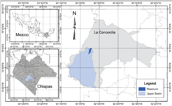
The upper basin of Cuxtepeques river, object of this study, is the one corresponding to the delimitation given by the watershed of the El Portillo II storage irrigation dam. Its basin is located in La Concordia, Chiapas in Mexico (Figure 1), between coordinates 15° 55' 00'' and 16° 00' 00'' of North latitude and 92' 53' 35'' and 92° 56' 25'' West longitude.
The micro-climate conditions in the basin vary according to the location, as in highest areas of the Sierra Madre there is temperate local climate with summer rain-fall, the middle zone presents a semi-warm humid and in the lowest sub-humid warm zone (Arellano, 2005).
The rainfall data with years with complete record, were taken from the station called Finca Cuxtepeques, because to its proximity with the Sierra Madre of Chiapas. In the period from 1953 to 2005 an average annual rainfall of 2,043.31 mm was obtained; with a minimum of 1,534.1 mm in 1953 and maximum in 2005 of 2,835.7 mm.
The basin's topography is characterized by mild slopes in the valley to very steep slopes in some points of the Sierra Madre. According to INEGI's edaphology information the main soil groups are: Leptosol, Acrisol and Luvisol which occupy about 90% of the basin surface.
Regarding the USLE developed by Wischmeier and Smith (1978), its parameters are shown in Equation 1 and each of these variables are described below:
For the present study, the almost inexistence of management practices for soil conservation was taken into consideration, so that the P factor has unit value, in each analysis scenario. The other parameters were obtained in some cases with modifications to the original methodology; they were made by different authors for the regional conditions of study site.
Factor of erosivity R was obtained through the equation given by Bauman and Arellano (2003):
Where: R is in MJ-mm-(ha-h-year)-1 and Pp is the annual mean rainfall in mm. This annual mean rainfall was calculated for the period between each study scenario, considering only continuous records of Finca Cuxtepeques gauging station.
The erodability soil factor (K) in (Ton-ha-h)-(MJ-mm-ha)-1 was obtained by consider the main soil group in each case. The K value was assigned from the World Reference Base (WRB) of the soil resource (FAO, 2006), according to tables showed by Arellano (1994).
In the other hand, the slope length-gradient factor (LS) was calculated with the product of L and S. The L factor was evaluated with the Equation 3 (Desmet and Govers, 1996):
Where: Aij is the contributing unitary area to the entrance of a pixel, D is the pixel size and X is a correcting form factor. The exponent m in Equation 3 was obtained with:
Where β is the slope in radians, obtained with the methodology proposed by (Castro, Lince and Riñao, 2017; Flores, et al., 2003).
The S factor was calculated apply the next criteria:
If
Then
In opposite case
The C factor of crop/vegetation (dimensionless) was obtained through satellite imagines, the Normalized Differential Vegetation Index (NDVI) was calculated and modifying the scale using the Equation 7, it was given by Durigón et al. (2014) and is called re-scaling C factor.
To determine the NDVI in each study scenario, multi-spectral imagines were employed and these corresponding to satellites Landsat 3 MSS (1980), Landsat 5 sensor TM (1998-1999) and 7 sensor ETM+ obtained from GloVis platform of the United States Geological Survey (USGS). The correction of the imagines was made using Erdas Imagine version 8.83. The Digital Elevation Model (DEM) was generated through a TIN from the topographic information in 1: 250,000 scale of National Institute of Statistic and Geography (INEGI, by its acronym in Spanish). The USLE parameters and their erosion rates in raster maps were made with Map Algebra technical (Arellano 1994; 2005; Pérez, 2013) and the Software ArcMap version 10.
The soil lost rates were defined according to the criteria of Arellano (2005); however, for this study it was decided to include a class adapted from the categories proposed by Pérez (2013), according to shown in Table 1. The weighted mean rates were obtained like the harmonic mean of values by grid in the erosion maps, and the annual means with to multiply this with the basin area to estimate the sediment rate (Gottschalk, 1964).
Table 1 Classification of water erosion rates.
| Erosion rates (Ton-ha-1-year-1) | Classification |
|---|---|
| 0-5 | Any |
| 5-10 | Incipient |
| 10-50 | Modérate |
| 50-200 | Severe |
| 200-1000 | Very Severe |
| >1000 | Extraordinary |
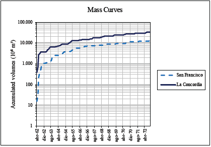
The behavior of the runoff volumes was analyzed with Flow-mass curve method or accumulated volumes for each gauging station of the basin.
For the analysis of the temporal variability of the flows, data of runoff volume and its solid fraction were used. The data correspond to gauging stations named San Francisco II and La Concordia, located inside the Cuxtepeques river basin, downstream from El Portillo II dam, from which eight years of continuous recording were obtained in the period from 1965 to 1973 agree with Secretaría de Recursos Hidráulicos (1972).
To determine the existence of regional homogeneity and the possibility of adjusting the data to a curve using the statistical regression procedure. Five more stations were selected, and two homogeneity tests were applied: Test of Discordance and Test S of Wiltshire (Campos 2010; 2011).
3. Results and Discussion
3.1. Estimation of Water Erosion in the Basin
Using ArcMap 10, the raster maps of USLE factors were generated. Applying the Equation 2 was obtained the R value for each study scenario (Table 2). The high R values are consistent because it is an area with high rainfalls and are analogous to those reported by Arellano (2005).
Table 2 Results got for the R factor.
| Scenario | Period of record by scenario | Pp (mm) | R factor (MJ∙mm)∙ (ha∙h∙year)-1 |
|---|---|---|---|
| 1980 | 1953-1976 | 1,887.56 | 20,812.13 |
| 1998 | 1981-1996 | 2,082.96 | 23,649.82 |
| 1999 | 1998 | 2,704.30 | 32,673.54 |
| 2003 | 1999 | 2,643.20 | 31,786.19 |
| 2006 | 2003-2005 | 2,382.75 | 28,003.67 |
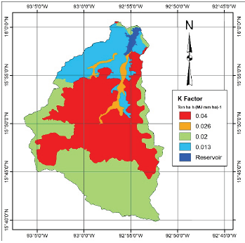
The soil erodability factor map (K) is showed in (Figure 2); it shows that the soils in the middle-high zone are more susceptible to erosion, with a K value of 0.04 (Ton-ha-h)-(MJ-mm-ha)1. While soils in valley have values less than 0.013 (Ton-ha-h)-(MJ-mm-ha)-1.
The Length-Slope factor (LS) is very important in the USLE model. As according to Arellano (1994) the LS factor (Figure 3) represents the spatial variability from erosion process and has effect both in the runoff volume and the surface velocity of the flow.
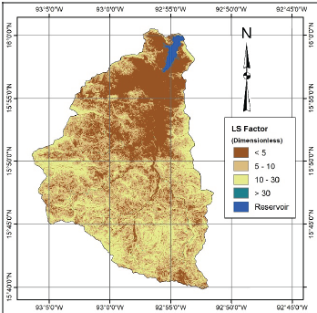
The map generated for LS factor (Figure 3) shows the spatial variability from basin relief. The values indicate a variation in low basin areas of 0-5, while in middle-high and high zones there are values from 5 to 30. Highest values are not common; however, these are numerically high, this mean that flow velocity is greater and thus also higher erosive capacity.
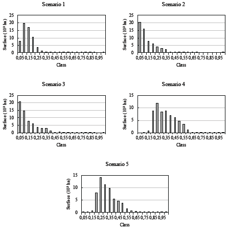
For the C factor, the data are showed in (Figure 4). The first study case (1980), point highest frequency in values less 0.2. In the other hand, the second scenario (1998) indicates a reduction of values; whose changes toward the third scenario (1999) are not of great relevance. In opposite side is the fourth scenery (2003), this shows a high increase of the factor, this tendency continues in the last scenario (2006), with important rises in some points, remain values of 0.2 and higher. With the Map Algebra technical, Equation 1 and ArcMap version 10, raster maps were made for each study scenario as shown in (Figure 5) for 1980.
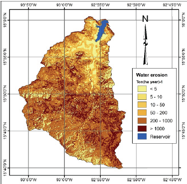
The results for the application of the USLE in five scenarios show important changes (Table 3 and Figure 6). In the first case, the less percent of affected surface corresponds to very low (5-10 Ton-ha-1-year-1) with 0.84% from basin area; while areas more affected with 51.16% and 17.41% correspond to very severe (200-1,000 Ton-ha-1-year-1) and extraordinary (>1,000 Ton-ha-1-year-1) rates, respectively.
Table 3 Erosion rate by affected area in five scenarios.
| Erosion rate† | Scenario 1 | Scenario 2 | Scenario 3 | Scenario 4 | Scenario 5 | |||||
|---|---|---|---|---|---|---|---|---|---|---|
| ha | % | ha | % | ha | % | Ha | % | ha | % | |
| <5 | 9,120.06 | 14.92 | 13,797.75 | 22.57 | 14,779.38 | 24.18 | 1,140.78 | 1.87 | 1,698.60 | 2.78 |
| 5-10 | 515.70 | 0.84 | 925 95 | 1.51 | 929.55 | 1.52 | 1,678.71 | 2.75 | 1,470.90 | 2.41 |
| 10-50 | 2,838.06 | 4.64 | 2,600.31 | 4.25 | 2,177.58 | 3.56 | 2,070.66 | 3.39 | 1,948.89 | 3.19 |
| 50-200 | 6,739.74 | 11 03 | 12,380.43 | 20 25 | 7,285.08 | 11 92 | 2,986.77 | 4 89 | 3,411.21 | 5.58 |
| 200-1000 | 31,2 73.74 | 51.16 | 26,126.31 | 42.74 | 26,351.49 | 43.11 | 13,144 71 | 21.50 | 16,153 68 | 26 42 |
| >1000 | 10,643.58 | 17.41 | 5,300.13 | 8.67 | 9,607.80 | 15.72 | 40,109.25 | 65.61 | 36,447.60 | 59.62 |
| Weighted mean† | 31.71 | 26.05 | 37.90 | 105.39 | 86.52 | |||||
| Annual mean‡ | 1.94 | 1.59 | 2.32 | 6.44 | 5.29 | |||||
Notes: † (Ton-ha-1 year-1), ‡ (Millions of Ton-year-1). Scenario 1 = November 1980 after of to fill the reservoir for first time; Scenario 2 = February 1998 before of the first extreme event; Scenario 3 = February 1999 after of the first extreme event; Scenario 4 = Abril 2003 before hurricane Stan; Scenario 5: February 2006 after of hurricane Stan.
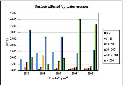
It is observed a decrease in erosion rates from the first to the second scenarios (1980-1998); in this period, the incipient erosion rate has the less percent with 1.51%, however, there is significant decrease in very severe and extraordinary rates with 42.74 and 8.67%, respectively.
The variation in some values in the third scenery (1999) is subtle, with changes almost imperceptible. The variation in very low and very severe rates showed increase of 0.01 and 0.37%. However, areas with extraordinary rates (>1,000 Ton-ha-x-year-1) increase to double the surface compared to the previous period (from 8.67% to 15.72%).
Also, the changes in last two scenarios (2003 to 2006) with respect to the three previous ones, are intensive and drastic, a lot of percent of the areas basin were affected by very severe and extraordinary erosion rates.
The fourth scenario (2003) shows that 65.61% of surface basin has reached extraordinary erosion rates, while rates less than de 200 Ton-ha-1-year-1 are almost 12.89%.
The last study scenario (2006) shows permanency in the same rates than the before one (2003), also there is a decrease in extraordinary rates, nearby 6% and an increase in the other categories.
The foregoing shows the impact of the extreme rainfall of the hydro-meteorological events of September 1998 and October 2005 on the basin water erosion. The annual mean and weighted water erosion rates estimated for each period, showed a constant increase in the areas affected with water erosion severe, progressive in some cases and drastic in other ones (Table 3 and Figure 6).
3.2. Adjustment of Runoff and Sediment Volumes in the Basin
The mass curves calculated for the two gauging stations (Figure 7) showed similar behaviors; even these have changes in their tendency in near dates. The most pronounced changes occurred between June 1962 and November 1963. In general, the turning points of the curve for the San Francisco II gauging station are two or three months behind La Concordia gauging station. Nevertheless, both curves have statistical homogeneity each other.
The regional homogeneity tests were applied to seven gauging stations, between them San Francisco II and La Concordia. The Discordance Test showed that none gauging station processed in this test has anomalous records. Although some values were high, the discordance Di generated through t ratios of L-moments from each one of records, is less than critical value Dc = 1.917.
A value of the statistic S = 9.297 was obtained in the Wiltshire Test, with regional variance VR = 0.0959 and weighted region-average value CVp = 0.3755. This test proves the existence of homogeneity in data series, as S is less than critical value X2c = 12.592 with six degree of freedom and a significance level of 5%. The results in both tests and the gauging stations used are shown in (Table 4).
Table 4 Results got of homogeneity tests.
| Gauging station | Code | Period (N° years) | t | t3 | t4 |
|---|---|---|---|---|---|
| Aquespala | 30102 | 1966-1984 (19) | 0.2099 | 0.1599 | 0.1462 |
| Argelia | 30040 | 1954-1974 (21) | 0.1533 | -0.0002 | 0.1353 |
| La Concordia | 30056 | 1956-1973 (18) | 0.2154 | 0.2116 | 0.0632 |
| El Salvador | 30048 | 1954-1973 (20) | 0.3096 | 0.0539 | -0.1483 |
| San Fco. I | 30033 | 1951-1963 (13) | 0.1638 | 0.0760 | 0.1564 |
| San Fco. II | 30091 | 1965-1979 (14) | 0.1989 | 0.2877 | 0.2377 |
| Sta. Isabel | 30053 | 1956-1973 (18) | 0.2408 | 0.3403 | 0.2971 |
| N | α | VR | CVp | S | DF |
| 7 | 0.05 | 0.0959 | 0.3755 | 9.2970 | 6.0 |
The homogeneity in the sub-region formed by the seven gauging stations is a good indicator to use these gaging data. Because inside the dam basin, there are only two gauging stations, it was made by regression: an adjustment from data set for several models.
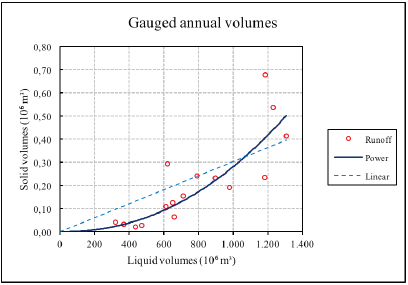
The best polynomial model was with grade six. However, this model had negative values in the function domain, so that it was choose a potential equation (Equation 8) with coefficient correlation r = 0.8835, that showed better adjustment with the data.
To compare with models shown by Krysanova et al. (2002) and Walling (2009) for different rivers in the world, it was made an adjustment with a linear equation at the origin (Equation 9). Where Vs is the solid volume in millions of m3 and V is liquid volume in millions of m3. The curves are shown in (Figure 8).
4. Conclusions
The integration of the USLE to SIG's is a very important tool to evaluate erosion rates at the basin level. The generation of raster maps with Map Algebra technical has been key for this objective. It is accepted that is essential the calibration of the USLE parameters in field, as this will contribute to obtain more sense results.
The changes in the vegetation cover in the basin and the rainfall intensity show a great relationship with variations in erosion rates in each study period. The basin susceptibility versus the water erosion has increased significantly, which is radically reflected in the scenarios from 1999 to 2003 that show the impact of rainfalls in Sept-ember 1998 that accelerated the severe water erosion in several areas.
The results show the need to establish support practices to improve the management conditions and vegetation, thus, to reduce its vulnerability to the impacts induced by extreme rainfalls and generated by the global climate change.
The homogeneity tests showed congruence with each other, giving favorable results. Both tests represent a significant reference for the flood regional analyst that can be applied to study the sedimentation in the basin.
Although the regression curve obtained shows a good fit to the data, it becomes clear that there is a need to have longer recording periods, since it will allow to know in detail the changes that the dynamics of the sediment production and the load have undergone suspension in the recent past.

