Luis A. Montes V.¹ and Andrés Cárdenas Contreras²

¹ Luis A. Montes V.: Geosciences Department, Universidad Nacional de Colombia, Bogotá, D.C. Colombia.
lamontesv@unal.edu.co
²Andrés Cárdenas Contreras: Engineering Faculty. Universidad Distrital Francisco José de Caldas, Bogotá, D.C. Colombia.
acardenas@udistrital.edu.co

ABSTRACT

Commonly seismic images are displayed in time domain because the model in depth can be known only in well logs. To produce seismic sections, pre and post stack processing approaches use time or depth velocity models whereas the common reflection method does not, instead it requires a set of parameters established for the first layer. A set of synthetic data of an anticline model, with sources and receivers placed on a flat topography, was used to observe the performance of this method. As result, a better reflector recovering compared against conventional processing sequence was observed.

The procedure was extended to real data, using a dataset acquired on a zone characterized by mild topography and quiet environment reflectors in the Eastern Colombia planes, observing an enhanced and a better continuity of the reflectors in the CRS stacked section.

Keywords: Seismic section, CRS, Multiparameter traveltime, Coherence Analysis.

RESUMEN

Las imágenes sísmicas son comunes en dominio del tiempo debido a que el modelo en profundidad se conoce solamente en registros de pozo; para producir las secciones sísmicas los enfoques de procesamiento antes y después de apilado usan modelos de velocidad en tiempo o profundidad no así el método de superficie común de reflexión que requiere de un conjunto de parámetros establecidos para la primera capa. Aplicada a datos sintéticos de un anticlinal con fuentes y detectores colocados sobre una superficie plana, el método exhibió un buen desempeño desplegando los reflectores más claramente que los suministrados por el procesamiento convencional. El procedimiento se aplicó a una línea sísmica adquirida en los Llanos Orientales Colombianos, en una zona caracterizada por suave topografía y reflectores de ambientes tranquilos, se observó un realce y mayor continuidad en los reflectores.

Palabras Claves: Sección sísmica, CRS, tiempo de tránsito multiparámetro, Análisis de coherencia.

INTRODUCTION

Recently a new approach has been developed to estimate a more approximate traveltime function through geometrical optics approximation. The approach is based in the Common Reflection Surface (CRS) method, supported on fictitious normal wave and normal incident point wave used to describe zero offset ray propagation (Tygel et al., 1997). The traveltime is expressed in terms of the emergence angle of this ray and the wave front curvatures of the two waves. The traveltime approximation was defined for 3D media and related with the kinematic attributes of the wave field. The method has been extended to study how offset affects amplitude by obtaining analytical curves (Biloti et al., 2002) to estimate velocity in depth (Ortega et al. 2003) and static corrections (Grossfeld et al, 2001).

The CRS method uses a set of multi-covering data acquired on a flat surface without assumption of horizontal parallel planar interfaces. In case of non planar surfaces, the dataset must be continued to flat datum before stacking process.

CRS TRAVELTIME FUNCTION

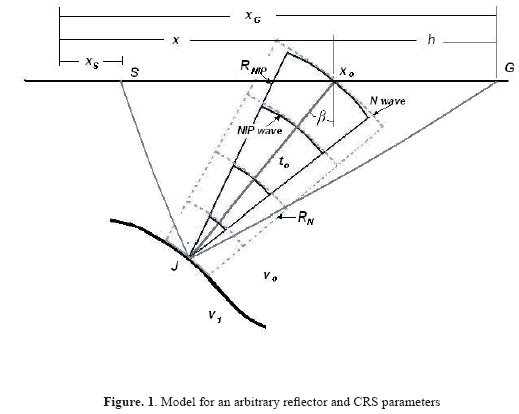
Figure 1 displays a v₀ velocity layer over a semi infinite v₁ velocity medium separated by a curved interface. The ray perpendicular to the reflector in J point (named normal ray) emerges with an angle β at x_o point spending t₀ to travel from x_o t_o J and back to xo (zero offset traveltime). Over the flat surface, the couple source-detector images the curved reflector through the ray that follows the trajectory S-J-G (called paraxial ray); hence, the traveltime function may be estimated dividing the path length of the ray by v₀ speed. In figure 1, two wave fronts are shown where the hypothetical N wave is generated by an exploding reflector with curvature radii R_N and the NIP wave is generated by a point source in R with curvature radii R_NIP. Both measured in the vicinity of the central ray. For the coordinate system fixed to the central ray, the square of the traveltime for the paraxial ray is approximated by Tygel et al. (1997):

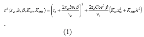
Here, the midpoint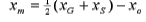 and the half offset

are pair coordinates defining a new vector space with β, K_N, and K_NIP CRS parameters. The last two parameters represent the wavefront curvature of both N wave and NIP wave respectively.

The CRS process flowchart contains the same steps presented in a conventional sequence up to NMO stack. This step is performed applying the move-out formula expressed in the multiparameter traveltime of the equation 1, providing a better ZO section of CRS parameters during the coherence analysis of the multiple shots and receivers data. Before using multiparameter traveltime it is necessary to be familiar with the near surface velocity model (e.g., to provide t₀ and v₀ values).

Model

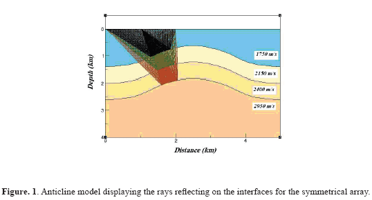
An anticline model of 5 km wide and 3 km depth with three layers over a semi infinite medium was build (Figure 2), and a synthetic dataset with 75 records with 40 m source interval and 20 m group interval was generated. A split spread geometry with 100 receivers and 25 maximum fold was used, where h varies from 5 to 505 m increasing 10 m and x ranges from 505 m to 4455 m increasing 10 m.

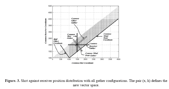
The map of shots against receivers coordinate distribution is displayed in Figure 3 with all gather configurations (e.g., common shot (CS), common receiver (CR), common mid point (CMP) and common offset (CO)). The new pair coordinates, Half-Offset and Mid Point, are linearly independent and define a new vector space, where the traveltime function as defined in equation 1 is established.

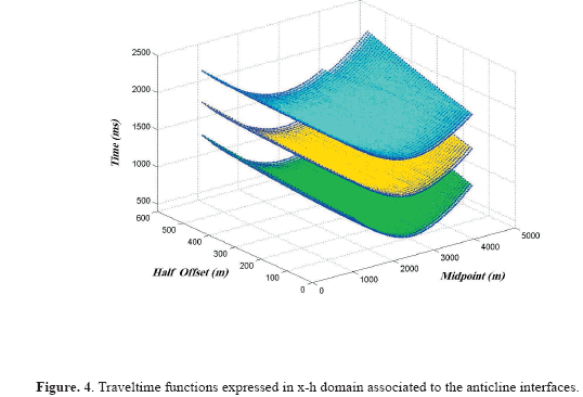
Conventional stacking assumes that reflections are represented by hyperbolic traveltime and reflectors by points. The CRS approach proposes that the recorded data has to be associated with common reflection surfaces, instead of common reflection points. Hence to stack the data, it may be focused to a common reflection surface using multiples shots and receivers, allowing the inclusion of more traces in the procedure. In figure 4 the surfaces represent the traveltime functions in x-h domain for three reflectors in the anticline model, recalling that for each point on reflector there is an associated CRS surface in this space.

FIRST INTERFACE PARAMETERS ESTIMATION

To solve the traveltime function, for the first layer, implies to know the parameters β, K_N, and K_NIP, whereas v₀ distribution can be established using depth hole and up-hole time of the shots usually available in seismic surveys, and t₀ values from ZO sections. Through three different configurations the expression 1 may be simplified as explained below.

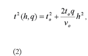
In common mid point setting, where the fixed point coincides with the middle point xm = 0, equation 1 is reduced to

On the other hand, in zero offset configuration h=0, equation 1 becomes:

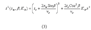
And finally in Common shot configuration, where x = h, equation 1 is simplified to

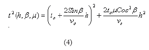
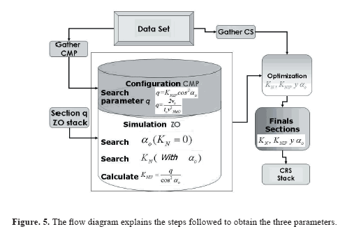
The equations 2, 3, and 4 are linearly independent with 3 unknown parameters β, R_N, and R_NIP which means that this system equation is solvable, and the simplified flow diagram shown in Figure 5 explains the procedure used to estimate them. In the first step, the parameter q = K_NIPCos²β is estimated in the multi-coverage data sorted in CMP configuration, according to equation 2. The β and K_N values are iteratively approximated, using K_N = 0 as initial setting in expression 3, and using this β value to know K_N, and so on. Finally, the third parameter is calculated through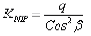

In Figure 6, the behavior of the q parameter for the first interface is plotted in vector space x-h. According to Biloti et al. (2001) this parameter may become imaginary depending on KNIP values, but in this case is always real. The traveltime for a horizontal flat reflector is 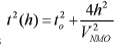and when it is compared with equation 2, allows to define the parameter 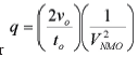which relates stacking velocity with CRS operators.

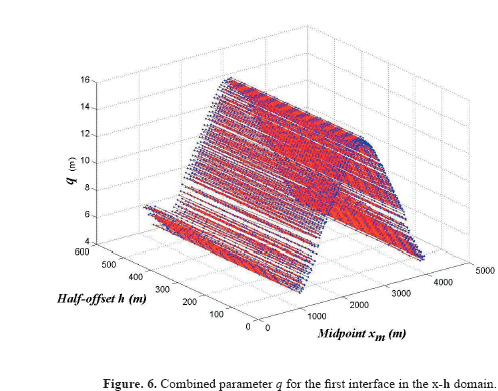
Figure 7 shows the behavior of emergence angle β for rays normal to the first interface. Its values range from -28º to 28º, being zero at the anticline’s apex.

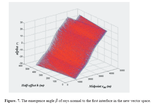
Although the K_N surface may set any real value, in this case is always positive as shown in Figure 8 where it ranges between 2.4510 E-004 and 5.2995E-004. Due to its small value, its contribution to equation 1 is too low compared with the other parameters.

In figure 9, the K_N behavior is depicted with values ranging from 0.0016e-004 to 9.7585e-004, recalling that by definition K_NIP = 0 corresponds to a flat reflector.

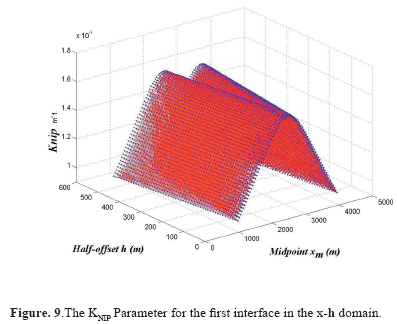
Figure 10 shows at the left a CDP gather, at the middle the same gather after NMO correction, and at the right the same gather after CRS correction. In the CMP domain, the two traveltime expressions are equivalent; therefore the two corrected gathers look similar, indicating the performance of CRS correction.

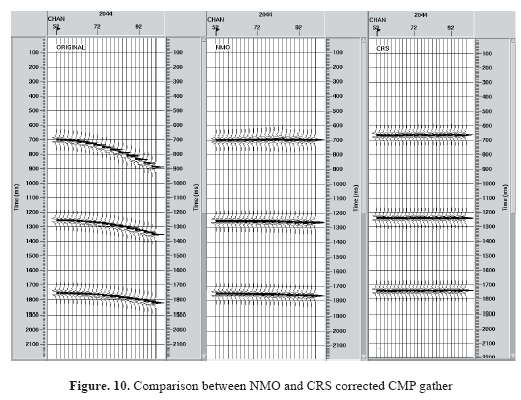
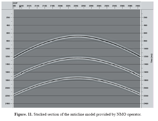
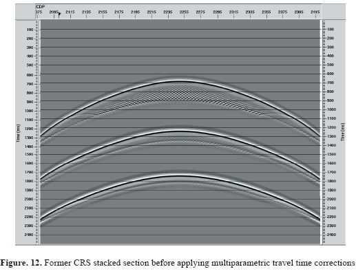
Figure 11 shows the NMO stacked sections with the three interfaces clearly displayed as expected. The figure 12 shows the former CRS stacked section with the reflectors correctly positioned in time, but with a blurred image. This effect decreases in depth. At this stage of the CRS process, the travel time correction has not been applied.

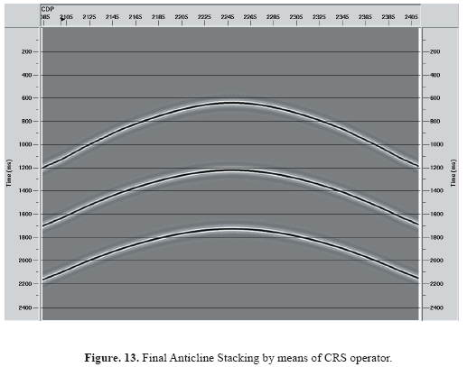
The Figure 13 shows the final stacked section provided by means of CRS operator, the events were enhanced and displaced to their correct position in time. Comparing the images provided by NMO and CRS techniques, a similar coherence is observed in the three reflectors, indicating the robust performance of CRS stacking method.

REAL DATA

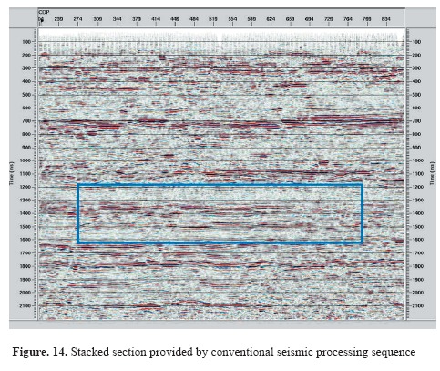
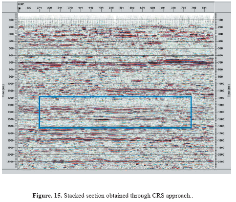
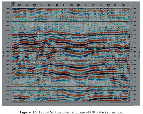
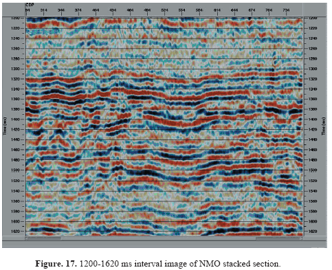
Tested on synthetic data, the next step was to apply the technique to real data using a high quality seismic dataset acquired on the eastern Colombian land plains. The dataset was processed using a conventional sequence and a final stacked section through NMO correction was obtained (see Figure 14). Following the same methodology explained for the anticline model, the parameters associated to the first layer were estimated and fed to the algorithm to provide the CRS stacked section displayed in Figure 15. According to the theory, in case of parallel plane interfaces, the normal emergence angle becomes zero and also K_N = 0, because the interfaces in the zone are considered flat. In order to get comparable images, the dataset was continued to a flat datum and the same residual static corrections were applied on both seismic processing sequences. As result, the deep reflectors in CRS stacked section are enhanced and a better continuity observed. The zones between 1200 – 1620 ms for both stacked images were zoomed and displayed in figures 16 and 17 in order to remark their differences. As can be observed, the CRS section increased the coherence in reflectors defining a better lateral continuity.

CONCLUSIONS

The anticline model studied shows the detailed behavior of the three parameters provided by CRS stacking. These results provide valuable information to be considered when the CRS operator technique is applied to real data.

The common reflection surface corresponds to an image built through the stacking of a number of seismic traces from different CMP gathers, in which the sources and receivers are close to the image point, and are corrected through the simulation of a ZO section. This is acceptable because in the x_m-h-t domain, traces are organized in such a way that it is possible to obtain a better approximation and quality in the seismic data processed thanks to the parameters triplet.

This method requires no knowledge of an underground model. It only requires the surficial velocity in the vicinity of stacked trace location and it can produce the simulation of a very precise ZO. In special cases where the topography is rather abrupt, it will be useful to define a more accurate geological model.

The CRS stacking method furnishes additional information through the three kinematic stacking parameters, making possible to define the interfaces, since their location, depth and curvature may be determined. The emergence angle and the NIP wave front curvature are the two most routinely used parameters to permit reverse tracing of rays.

The CRS method guarantees that through analytical expressions based on the spherical representation of wave fronts, overtime correction is described for a given source-receiver pair with respect to the trace of a ZO image. Determining the triplet of parameters requires larger computational effort but it provides a better ZO sections with enhanced and more continuous reflectors as displayed in CRS stacked sections of real data. The obtained results encourage CRS research in an effort to improve the performance of the algorithm to apply this technique to any seismic line.

ACKNOWLEDGEMENTS

The authors wish to thank the Geophysics Group of the Universidad Nacional de Colombia-Bogota and its Department of Geosciences for the support given to the CRS research project. Also, we express our grateful to Halliburton Inc for the provided software used along the research and the anonymous reviewers who contribute with their suggestions.

REFERENCES

Biloti R., Santos, L., and Tygel M. (2001). Multiparametric traveltimes: estimation and inversion. Ph.D. thesis, State University of Campinas, Brazil (in Portuguese).        [ Links ]

Grossfeld V. (2001). Correction of topographic effect in seismic data using multiparameter traveltime formulas. Master thesis, State University of Campinas, Brazil (in Portuguese).        [ Links ]

Hubral P. and Krey, T. (1980). Interval Velocities from seismic reflection traveltime measurements. SEG.        [ Links ]

Ortega, C. and Montes, L. (2003). Depth velocity model estimated through the diffraction function: a real data application. Geofísica Colombiana. 61-64. (in Spanish).        [ Links ]

Tygel M., Hubral, P., and Schleicher, J. (1997). Eigenwave based multiparameter traveltime expansions. Ann. Int. Mtg. SEG. Expanded abstracts, 1770-1773.        [ Links ]

Vieth K. (2001). Kinematic wavefield attributes in seismic imaging. Ph.D. thesis, Karlsruhe University, Germany.        [ Links ]