Awni T. Batayneh.

Department of Geology, King Saud University , PO Box 2455 , Riyadh 11451 , Saudi Arabia
Corresponding author. Tel.: ++966-56-8086395.
E-mail address: awni_batayneh@yahoo.com (A. T. Batayneh)

Manuscript received July 8 2007. Accepted for publication December 10 2007.

ABSTRACT

During 2006, geoelectrical measurements using the vertical electrical sounding (VES) method were conducted on the eastern Red Sea coast in Jordan, using the SYSCAL-R2 resistivity instrument. The objectives of the study were (i) to evaluate the possibility of mapping of Quaternary sediments medium in areas where little is known about the subsurface geology and to infer shallow geological structure from the electrical interpretation, and (ii) to identify formations that may present fresh aquifer waters, and subsequently to estimate the relationship between groundwater resources and geological structures. Data collected at 47 locations were interpreted first with curve matching techniques, using theoretically calculated master curves, in conjunction with the auxiliary curves. The initial earth models were second checked and reinterpreted using a 1-D inversion program (i.e., RESIX-IP) in order to obtain final earth models. The final layer parameters (thicknesses and resistivities) were then pieced together along survey lines to make electrical cross sections. Resistivity measurements show a dominant trend of decreasing resistivity (thus increasing salinity) with depth and westward toward the Red Sea. Accordingly, three zones with different resistivity values were detected, corresponding to three different bearing formations: (i) a water-bearing formation in the west containing Red Sea saltwater; (ii) a transition zone of clay and clayey sand thick formation; (iii) stratas saturated with fresh groundwater in the east disturbed by the presence of clay and clayey sand horizons. Deep borehole (131 m) drilled in the northwestern part of the study area for groundwater investigation, has confirmed the findings of the resistivity survey.

Key words: Red Sea coast; Geoelectrical measurements; Geology; Hydrogeology; Jordan.

RESUMEN

Durante 2006, mediciones geoeléctricas que usaban el método eléctrico vertical de sondeo (EVS) fueron realizadas en la costa oriental del mar rojo en Jordania, usando el instrumento de resistividad SYSCAL-R2. Los objetivos del estudio fueron (i) evaluar la posibilidad de cartografiar los sedimentos cuaternarios en áreas donde poco se sabe sobre la geología subterránea y deducir estructuras geológicas someras a partir de interpretación eléctrica, y (ii) identificar formaciones que pueden presentar acuíferos, y posteriormente estimar la relación entre recursos de agua subterránea y estructuras geológicas. Los datos recolectados en 47 sitios fueron interpretados primero con técnicas para emparejar las curvas, usando curvas principales teóricamente calculadas, conjuntamente con las curvas auxiliares. Los modelos iniciales terrestres fueron comprobados y reinterpretados en segundo lugar usando un programa de inversión 1-D (i.e., RESIX-IP) para obtener modelos finales terrestres. Los parámetros finales de la capa (espesores y resistividades) entonces fueron ensamblados a lo largo de líneas de medición para hacer secciones transversales eléctricas. Las mediciones de resistividad demuestran una tendencia dominante de disminución de la resistividad (además incremento de la salinidad) con la profundidad y hacia el oeste del mar rojo. Por consiguiente, tres zonas con diversos valores de resistividad fueron detectadas, correspondiendo a tres diferentes formaciones portadoras: (i) una formación acuífera en el oeste que contiene el agua salada del mar rojo; (ii) una zona de transición entre arcilla y arena gruesa arcillosa; y (iii) estratos saturados con agua subterránea fresca en el este con presencia de arcilla y horizontes arcillosos arenosos. Pozos (131 m) perforados en la parte noroccidental del área del estudio para la investigación de agua subterránea, han confirmado los resultados.

Palabras claves: Costa del Mar Rojo; Mediciones Geoeléctricas; Geología; Hidrogeología; Jordan.

The problem of the salination of groundwater aquifers arises in coastal areas, where the excessive pumping of unconfined coastal aquifers by water wells leads to the intrusion of sea water. This negative effect of human activity has been recorded in many areas of the world. Hence, this problem is likely to arise in areas like Jordan that has poor water resources (low
precipitation and high evapotranspiration) and has mismanagement of water resources (e.g., Batayneh, 2006; Batayneh and Qassas, 2006).

Jordan is considered as one of the ten poorest countries in water in the world. An arid climate, high natural growth rates, and forced migrations have conspired to push available water resources to the limit. Annual rainfall in Jordan ranges from 600 mm in the northwestern highlands to less than 100 mm in the eastern and southern regions. It is estimated that 80.6% of Jordan receives less than 100 mm of rainfall per year (Salameh and Bannayan, 1993). Assuming that the average rainfall in this area is 70 mm, dry areas in Jordan receive 5 billion m3 a year. Most of this water flows in small drainage basins or wadis to end up in playas (qa’s), and ultimately are lost to evaporation.

Due to the scarcity of boreholes in the east area of the Red Sea coast in Jordan which could provide information on the configuration of the different water bodies, vertical electrical sounding (VES) survey, utilizing a Schlumberger array configuration, SYSCAL-R2 resistivity instrument (IRIS Instruments, France), were performed on 47 sites for several purposes: (1) verification of the presence of the different water-bearing formations and estimation of their depth and thickness; (2) finding the relationship between the resistivity variations and the different configurations of the water-bearing formations; and (3) mapping the water table in the shallow coastal aquifer and selecting new location(s) for drilling.

Data from a single shallow (33 m) borehole (K1, Fig. 1) drilled by the Jordan Phosphate Mines Company showed saline water (TDS > 30,000 mg/l) at 32 m deep, and a 131 m deep borehole (K3028, Fig. 1) drilled by the Water Authority of Jordan for groundwater investigation encountered saline water (TDS > 27,000 mg/l) at 127.5 m deep. The data were analyzed and used to correlate the results of the geoelectrical surveys (see section field measurements and methods of interpretation). The K1 shallow borehole penetrated alternating bands of gravel and sand down to a depth of about 4 m which is underlain by a unit composed by approximately 25 m clay and clayey sand sediments. The third unit corresponds to the sand/sandy clay containing saline water (saturated). Data fromthe K3028 deep borehole shows that three units of sediments were found. The upper unit has approximately a thickness 36.5 m and consists of medium to coarse grained size gravel and sand. The underlying 91 m thick unit is mainly composed by clay and clayish sand. The third unit is composed by sand/sandy-clay sediments containing saline water (saturated).

STUDY AREA

The area under study is approximately located at 30 km to the south of Aqaba city in the southwestern part of Jordan. It is limited to the south by the Jordanian-Saudi border and to the west by the Red Sea (Fig. 1).

The study area is located in an extremely arid environment with an annual average precipitation of 70 mm. Rainfall generally occurs during the winter months (November to January). However, there are years where the rainfall is absent; while
in other years, ephemeral floods of short duration may occur. The climate of the region is very hot in summer (April to August) with temperatures exceeding 38 ºC in summer (April to August).

The area under investigation was included in the 1:50,000 national geological mapping project carried out by the Geological Mapping Division of the Natural Resources Authority of Jordan (al Khatib, 1987). This map shows that metamorphic rocks of the late Proterozoic Aqaba Complex dominate the eastern side of the study area (Fig. 1). It varies in composition from monzogranite to alkali feldspar granite. The coastal plain between the metamorphic rocks and the Red Sea consists mainly of Quaternary continental sediments. These constitute clastics (clay, sand, and gravel) deposited in fan deltas, with some intercalations of lacustrine sediments (clay, gypsum, and aragonite) of Pleistocene age (al Khatib, 1987). The coastal plain area (Fig. 1) is approximately 7 km long and 9 km wide and is accessible from a modern highway joining Jordan with Saudi Arabia.

The alluvial shallow aquifer is the primary source of water for domestic, municipal, and industrial use in the region. The recharge to this aquifer takes place either along the elevated areas in the east and northeast sides, or due to local surface water infiltrations.

FIELD MEASUREMENTS AND METHODS OF INTERPRETATIONS

Surface resistivity methods have been used for groundwater research for many years. Earth resistivities are related to important geologic parameters of the subsurface including types of rocks and soils, porosity, and degree of saturation (Keller and Frischknecht, 1966). It was shown by Parasnis (1956 and 1966) that the electrical resistivity of rocks and minerals, except for massive sulfides and graphite, vary in a wide range between 1 to 107 ohm-m, whereas coastal aquifers that are prone to saline water are identified by relatively low resistivity values. Thus, saltwater can be easily distinguished from almost any combination of lithological types. Resistivity methods are used to map the freshwater-saltwater interface and for studying conductive bodies of hydrogeological interest (e.g., Zohdy and Jackson, 1969; Ayers, 1989; Barongo and Palacky, 1991; Khair and Skokan, 1998; Gnanasundar and Elango, 1999; Mukhtar et al., 2000; Batayneh, 2006).

In general, the resistivity method involves measuring the electrical resistivity of earth materials by introducing an electrical current
into the ground and monitoring the potential field developed by the current. The most commonly used electrode configuration for geoelectrical soundings, which was used in this field survey, is the Schlumberger array. Four electrodes (two current A and B and two potential M and N) are placed along a straight line on the land surface such that the outside (current) electrode distance (AB) is equal to or greater than five times the inside (potential) electrode distance (MN). Vertical sounding, in Schlumberger array, were performed by keeping the electrode array centered over a field station while increasing the spacing between the current electrodes, thus increasing the depth of investigation.

The potential difference (ΔV) and the electrical current (I) are measured for electrode spacing and the apparent resistivity (ρa) is calculated by the equation:

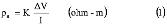
is the geometrical factor that depends on the electrode arrangement for the Schlumberger array.

A total of 47 VES stations were established across the study area. The data were collected using a SYSCAL-R2 resistivity instrument (IRIS Instrument, France). The layout of the survey stations is superimposed on the geological map in Figure 1. The locations of the VES sites were considerably restricted by logistical difficulties. The presence of narrow valleys and topography prevented a wider coverage. The maximum AB/2 spacing of the Schlumberger array ranged from 15 m to 900 m. The separation of the current electrodes was = 3, 4, 6, 8, 10, 12, 16, 20, 24, 30, 40, 50, 60, 80, 100, 150, 200, 250, 300, 350, 400, 500, 600, 800, 1000, 1200, 1400, 1600, and 1800 m. The potential electrode separation was = 1, 10, 20 and 40 m. The increase of the potential electrode separation MN allowed that readings from the same current electrode spread AB with the previous and expanded MN were taken.

The sounding curves were subjected to a preliminary interpretation using the partial curve matching technique by Zohdy (1965), and Orellana and Mooney (1966). Based on this preliminary interpretation, initial estimates of the resistivities and thickness (layer parameters) of the various geoelectric layers were obtained. In a second analysis method, the layer parameters derived from the graphical curve matching was then used to interpret the sounding data in terms of the final layer parameters through a 1-D inversion technique (e.g., RESIX-IP, Interpex Limited, Golden, Co., USA). Inversion analyses of the sounding curves have been made with an average fitting error of about 5%.

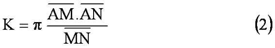
Quantitative interpretation of geoelectrical sounding curves is complicated due to the well known principle of equivalence (Van Overmeeren, 1989). Data from the K3028 borehole (Fig. 1) was used to minimize the choice of equivalent models by fixing thicknesses and depths to certain levels, and allowing the adjustment of resistivity. Correlation between VES stations 4 and 5 and lithology from the K3028 borehole was performed (Fig. 2) in order to determine the electrical characteristics of the rock units with depth.

Based on the lithological log from the K3028 borehole, the geological interpretation of the geoelectrical model for VES 4 and VES 5 (Fig. 2) is: (i) a resistive layer (500-1700 ohm-m) with variable thickness and moisture content at the surface, which consists of a mixture of gravel, silt, and sand; (ii) a thick clay and clayish sand layer having resistivity values of 30 to 40 ohm-m; and (iii) a saturated sandy layer with saline water having resistivity values of 1 to 10 ohm-m.

FIELD RESULTS

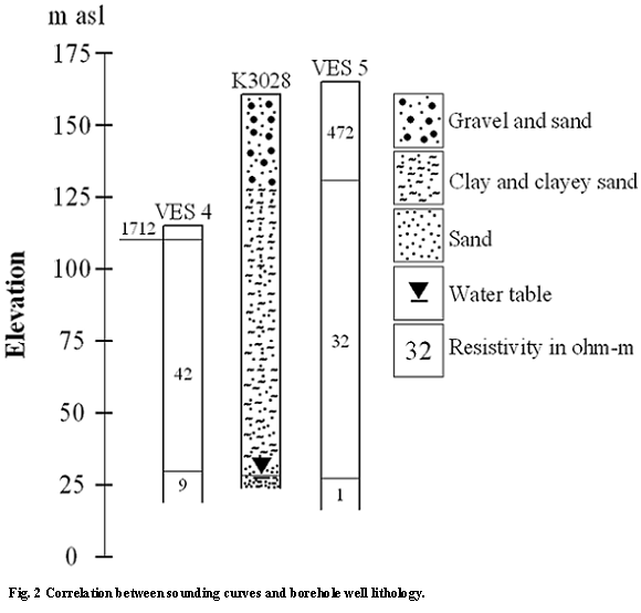
Analysis of VES curves Due to the distinctive characteristics features in the field of the apparent resistivity curves, the VES stations show four types of curves: Type I, Type II, Type III, and Type IV (Figure 3). These types were defined in terms of the number of geoelectrical layers and their respective resistivity relationships. Among the four types of curves, Type I and Type II curves show similar shape of field curves with layer resistivities decreasing with depth such that ρ1>ρ2>ρ3. Such curve behaviour undoubtedly proves the presence of a low-resistivity layer at the bottom of the section. Of the 47 field curves, 19 field curves at VES stations 1, 2, 3, 4, 5, 6, 7, 8, 9, 10, 11, 20, 21, 22, 28, 29, 30, 38, and 39 were classified as Type I (Figure 3a), and 15 of the field curves at VES stations 12, 13, 18, 19, 24, 25, 26, 27, 36, 37, 43, 44, 45, 46, and 47 were classified as Type II (Figure 3b).

Eight of the field curves at VES stations 15, 16, 17, 31, 32, 33, 34, and 35 were classified as Type III and reflect the presence of five geoelectric layers where the layers resistivity relationship is ρ1>ρ2<ρ3>ρ4<ρ5 (Figure 3c). The remaining five field curves at VES stations 14, 23, 40, 41, and 42 made in the eastern and southeastern parts of the study area were classified as Type IV and reflect the presence of three geoelectric layers where the layers resistivity relationship isρ1>ρ2<ρ3 (Figure 3d).

It is to be noted that the apparent resistivity values representing the surface layer in the four types of field curves vary considerably at different VES locations, mainly due to the fact that resistivity depends on the soil moisture content. The analysis of each type of curve in relation to groundwater in the study area is discussed in detail in the following sections.

Type I

The Type I curve (Figure 3a) generally shows: (1) a relatively thin surface layer of coarse grained loose sand, gravel, and sand dune existing below the ground surface having apparent resistivity of 300 to 1800 ohm-m, followed by (2) the presence of sand, clay, sandy clay, and gravel of varying grain size (fine to medium) of 50- 300 ohm-m apparent resistivity; and (3) a lowresistivity third layer with apparent resistivity < 12 ohm-m, indicating saline water. The Type I curves were obtained from soundings measured in the western side of the study area (Fig. 1).

Type II

The Type II curve (Figure 3b) is composed by (1) a thin layer of medium to coarse grained sand and gravel (surface layer) with an apparent resistivity of about 250 to 1300 ohm-m, (2) a second fine to medium grain size sand and gravel layer (100- 500 ohm-m), and (3) a relatively low-resistivity third layer (20-100 ohm-m) indicating a clay and clayish sand formation. The fields curves of Type II are obtained in the north-northeast trending narrow zone located to the east of the Type I curve (Fig. 1).

Type III

The Type III curves (Figure 3c) were obtained from soundings taken from profiles II and IV. Apparent resistivity values of these curves are relatively low, when compared to the other three types. The Type III field curves describe qualitatively a model composed of five layers where the layer resistivity relationship is ρ1>ρ2<ρ3>ρ4<ρ5.

From the top to the bottom, these are: (1) a sandy, clayish sand, and gravel of fine grained size having apparent resistivity of 60 to 250 ohm-m, followed by (2) the presence of clay and clayish sand formation (40-80 ohm-m), a (3) saturated sand with good groundwater quality (100 to 200 ohm-m), (4) a clay and clayish sand formation (40-80 ohm-m), and (5) a sandy formation saturated with fresh groundwater (80- 200 ohm-m).

Type IV

The Type IV sounding curves (Figure 3d) describe qualitatively a model composed by (1) a relatively thin surface layer with an apparent resistivity of 200 to 1300 ohm-m of medium to coarse grained material with a variable moisture content, followed by (2) the presence of a relatively low-resistivity second layer (40- 80 ohm-m), indicating a clay and clayish sand formation, and (3) a sandy formation saturated with fresh groundwater (100-200 ohm-m). The apparent resistivity values increase with depth from 100 to 200 ohm-m depending on the saturated condition.

bestfit model for four sounding data corresponding to the four types of field curves (I, II, III, and IV; Figure 3). It is of interest to note that the soundings of Fig. 4a were derived from the western part (site 1, Type I); Fig. 4b is based on sounding (site 37, Type II); Fig. 4c is based on sounding (site 33, Type III); Fig. 4d is based on sounding in the southeastern (site 41, Type IV) side. The best-fit models are derived along geoelectrical soundings points with lower and upper bound models (1-5% error). To the left of Fig. 4, it is shown the Schlumberger apparent resistivity curve with data (points) superimposed on the best match 1-D inversion (solid line). To the left of Fig. 4, the interpreted results in terms of resistivity and depth together with the allowable of equivalence (dashed lines) are shown.

Electrical cros sections

The results from the 1-D inversion of the geoelectrical soundings were compiled and plotted along two typical profiles: A-A’ and B-B’(Fig. 1). In these sections, the thickness of the subsurface layers and their geological structures are given. Two interpreted resistivity vs. depth cross sections are shown in Figs. 5 and 6.

Cross section A-A’ (Fig. 5) represents the behaviour of the northern side of the studied area. The distribution of the resistivity along the geoelectrical profile indicates the presence of two zones with different properties: the first zone is from sounding point 1 to 11 corresponding to Type I field curves and the second is from 12 to 13 representing Type II field curves. As seen in Fig. 5, the first zone shows resistivity values in the range 400-1800 ohm-m at the surface, which are considered caused by coarse grained sand, gravel, and sand dune at 3-50 m depth. In general, the layer thickness increases with increasing distance from the coast, followed by the presence of a relatively conductive second clay and clayish sand layer, ranging from 20 to 100 ohm-m, at shallower depths and thickening landwards. The top of this layer is above mean
sea level (MSL), by several hundred meters at sites 7, 8, 9, 10, and 11 (Fig. 5), followed by conductive layer with resistivity values of 1 to 11 ohm-m corresponding to saline water. The depth of this conductor is closed to MSL at coastal sites and show increasing depth with increasing distance from the coast. In the second zone shown in Fig. 5 (sites 12 and 13), the range is from 400-600 ohm-m and 5 to 15 m thick at the surface, which are considered caused by sand and gravel of varying grain size, followed by the presence of sand and sandy clay having resistivity values of 200 to 300 ohm-m and 10 to 30 m thick, followed by the presence of a relatively conductive third clay and clayish sand layer that has a resitivity value of 40 ohm-m at shallower depths.

Cross section B-B’ (Fig. 6) represents the behaviour of the southern part of the studied area. The cross section shows three different zones with different properties: the first zone is from sounding point 39 to 38 (Type I field curves), while the second zone from 37 to 36 (Type II field curves) and the third zone from 35 to 31 (Type III field curves). The first zone shows resistivity values in the range 500-600 ohm-m at the surface, considered to have been caused by coarse grained sand, gravel and sand dune at 10-20 m depth, followed by the presence of a relatively conductive second clay and clayish sand layer, ranging from 30 to 90 ohm-m, at shallower depths and thickening landwards, followed by conductive layer with resistivities of 2 to 3 ohm-m corresponding to saline water. In the second zone (Fig. 6, sites 37 and 36), the range is from 200-600 ohm-m and 40 to 50 m thick at the surface, considered to have been caused by sand and gravel of varying grain size (fine to medium), followed by the presence of sand and sandy clay having resistivity values of 80 to 100 ohm-m and about 100 m thick, followed by the presence of a relatively conductive third clay and clayish sand layer that has a 30 ohm-m resistivity value. In the third zone (Fig. 6, sites 35, 34, 33, 32 and 31), the main features of the derived structure, from the surface downward, may be summarized as follows: (1) a relatively thin surface layer of fine to medium sand, gravel, and sand clay that has a 100-300 ohm-m resistivity value and 5-15 m thick, followed by (2) the presence of clay and clayish sand having resistivity values of 50 to 90 ohm-m and 30 to 40 m thick, followed by (3) saturated sand with good groundwater quality having resistivity values of 100 to 270 ohm-m and 40 to 80 m thick; (4) a clay and clayish sand formation (50-80 ohm-m resistivity values and 40-90 m thick), and (5) a sandy formation saturated with fresh groundwater (100-350 ohm-m).

As seen from Fig. 6, the cross section is characterized by low to moderate resistivity values at the surface when compared with the cross section (Fig. 5). This decrease in resistivity values from about several hundred ohm meters on the surface along profile A-A’ to less than 650 ohm-m on the surface along profile B-B’ can be explained by more homogenous gravel and clayish sand nature of the Pleistocene sediments in the southern parts than the northern parts.

Geological and hydrogeological discusion

As seen before, the geoelectrical stratification of the study area comprises three to five units of high-, relatively high, relatively low-, and low-resistivity values from the surface down.

The western part of the study area (VES sites 1-11, profile A-A’, Fig. 5) can be easily interpreted directly in terms of geological and hydrogeological structures: a thin resistive coarse grained sand and gravel underlain by some tens of meters thick strata of fine to medium grain sand, gravel, clay, and clayish sand, followed by saltwater. As indicated by the cross section of profile B-B’ (Fig. 6), the basic structure beneath the central part of the study area (VES sites 37- 36 profile B-B’, Fig. 6) comprises three units of moderate high, relatively low, and low resistivity values from the surface down. The surface resistive layer represents dry sand and gravel. The second layer, marked by resistivities of some tens of ohm meters could indicate the presence of sand and sandy clay. The low resistivities values (~30 ohm-m) in the third layer may be related to the presence of clay and clayish sand layer. In addition, the eastern part of the study area (VES sites 35-31, profile B-B’, Fig. 6) comprises a succession of clay and clayish sand with fresh groundwater.

The use of VES surveying technique was proved useful to map the subsurface of structurally complex area where little geologic information is available due to lack of drillholes. VES surveys can also be used to locate bodies of groundwater and zones with anomalous electrical properties. The apparent resistivities measured on the study area can be explained by resistivity distributions involving four extensive electrically distinctive zones (I-IV, Fig. 7).

The study area can then be subdivided in four compartments (Fig. 7). Electrical differences between the four zones cannot be explained by water content, as different geological contexts have to be considered. As a result, two different hydrogeological behaviours can be distinguished: (i) a saline groundwater coastal aquifer in the western part, and (ii) a fresh groundwater aquifer in the eastern part.

An important general result of this study is the existence of different coastal hydrogeological zones directly linked to geological subsurface structures, despite a monotonic surface cover the surface alluvial and wadi sediments. The geological structures of coastal areas within an active plate may significantly control the groundwater behaviour and knowledge of the tectonic history of the region; therefore, it is necessary to deal with its hydrogeology. The second important result is that the area is characterized by a thick clay and poorly permeable substratum that occurs in the central part. This result provides new ideas about the hydrogeology of the area. The results obtained are in a good agreement with the borehole data available.

The author wishes to acknowledge the support received by the Natural Resources Authority of Jordan, IRIS SYSCAL-R2 resistivity equipment. Facilities provided by the Geophysics Division of the Natural Resources Authority of Jordan are acknowledged.

1. al Khatib, F., 1987. The geology of Jabal Al Mubarak & Al Yamaniyya. Map sheet nos. 3048 IV & 2948 I. Geological Mapping Division, Natural Resources Authority, Amman, Jordan.        [ Links ]

2. Ayers, J., 1989. Conjunctive use of geophysical and geological data in the study of an alluvial aquifer. Ground water 27: 625-632.        [ Links ]

3. Barongo, J., and Palacky, G., 1991. Investigations of electrical properties of weathered layers in the Yala area, western Kenya, using resistivity soundings. Geophysics 56: 133-138.        [ Links ]

4. Batayneh, A., 2006. Use of electrical resistivity methods for detecting subsurface fresh and saline water and delineating their interfacial configuration: a case study of the eastern Dead Sea coastal aquifers, Jordan. Hydrogeology Journal 14: 1277-1283.        [ Links ]

5. Batayneh, A., and Qassas, H., 2006. Changes in quality of groundwater with seasonal fluctuations: an example from Ghor Safi area, southern Dead Sea coastal aquifers, Jordan. Journal of Environmental Sciences 18: 263-269.        [ Links ]

6. Gnanasundar D, Elango L (1999) Groundwater quality assessment of a coastal aquifer using geoelectrical techniques. Journal of Environmental Hydrology 7: Paper 2        [ Links ]

7. Keller, G., and Frischknecht, F., 1966. Electrical methods in geophysical prospecting, Pergamon, NY.        [ Links ]

8. Khair, K., and Skokan, C., 1998. A model study of the effect of salination on groundwater resistivity. Journal of Environmental Geophysics 2: 223-231.        [ Links ]

9. Mukhtar, A., Sulaiman, W., Ibrahim, S., Abdul Latif, P., and Hanafi, M., 2000. Detection of groundwater pollution using resistivity imaging at Seri Petaling landfill, Malaysia. Journal of Environmental Hydrology 8: Paper 3.        [ Links ]

10. Orellana, E., and Mooney, H., 1966. Master tables and curves for vertical electrical sounding over layered structures. Interciencia, Madrid.         [ Links ]

11. Parasnis, D., 1956. The electrical resistivity of some sulphide and oxide minerals and their ores. Geophysical Prospecting 4: 249-279.        [ Links ]

12. Parasnis, D., 1966. Mining geophysics. Elsevier Science, Amsterdam.        [ Links ]

13. Salameh, E., and Bannayan, H., 1993. Water resources of Jordan, present status and future potentials. Fredrich Eberet Stiftung, Amman.        [ Links ]

14. Van Overmeeren, R., 1989. Aquifer boundaries explored by geoelectrical measurements in the coastal plain of Yemen. A case study of equivalence. Geophysics 54: 38-48.        [ Links ]

15. Zohdy, A., 1965. The auxiliary point method of electrical sounding interpretation, and its relationship to the Dar Zarrouk parameters. Geophysics 30: 644-660.        [ Links ]

16. Zohdy, A., and Jackson, D., 1969. Application of deep electrical soundings for groundwater exploration in Hawaii. Geophysics 34: 584-600.        [ Links ]