In electrical prospecting, the coefficient of anisotropy has been used to prove that rocks are stratified, such that the current flowing through them has different values in different directions. The application of coefficient of anisotropy in magneto-telluric prospecting has not been widely demonstrated. According to Telford et al., (1990), the geometrical arrangement of interstices in rocks has a pronounced effect on their conductivity. Because of the water contained in these interstices, the conduction tends to be electrolytic rather than ohmic. The resistivity of the rocks therefore varies with the mobility, concentration and degree of dissociation of ions in the interstices, which also depends on the dielectric constant of the solvent. If the propagation of current is in all directions, the medium is isotropic. When a medium is isotropic, it also means that the properties of the medium do not depend on the direction in which the stress is applied (Badgley, 1965). For example, sedimentary rocks are to some extent usually considered isotropic. However, generally, rocks are layered such that their elastic properties vary depending on the direction of deposition. If the conductivity depends on the direction of the current, the medium is anisotropic (Vozoff, 1990)

Thus, the anisotropy of rocks and rockmaterials is characteristic of their stratification (Telford et al., 1990). This is brought about by the fact that, for a homogeneous subsurface, telluric current tends to flow in the direction of strike of the bedding planeswhich is more conductive than in a direction perpendicular to it, which is more resistive. Therefore, according to Telford et al., (1990), the geometrical arrangement of the interstices in rocks also has a pronounced effect on their anisotropy.Vozoff (1990) goes further to say that in all laminated rocks, the laminae have differen resistivities, which he calls, micro-anisotropy. Employing the magnetotelluric method in the field, we came across rocks that are laterally isotropic, in which there is isotropy in one lateral direction and anisotropy in the perpendicular direction. For this reason, a value of apparent resistivity is always taken for each direction. Ritz (1982) also showed that in the interpretation using 2-D method, it is found that the apparent resistivity varies smoothly for currents flowing along the strike, but varies discontinuously with current across the strike. A particular example exists in metamorphic rocks such as the schist where rocks pile up in layers with the isotropic properties varying from layer to layer and the piled up layers behaving as if they were transversally anisotropic (Postma, 1955; Uhrig and Van Melle, 1955). The measurement of the elastic constant in these rocks often yield values which depend on the direction of measurement and differences of from 20 to 25% have been reported between measurements parallel and those perpendicular to the bedding planes (Telford et al., 1990).

2. Equation for the coefficient of anisotropy

For an isotropic medium, related equations of coefficient of anisotropy are simple and easily derived. We consider anisotropic and tabular media in which the values of apparent resistivity in a direction perpendicular to the structural discontinuity are higher than those parallel to it. These are called transverse apparent (ρ_t) and longitudinal (ρ_l) apparent resistivity respectively. To describe the geo-electric section of such a layered earth, Frischknecht and Keller (1966) considered a layer with a cross-sectional area of one square metre, a specific resistivity ρ_i, but varying thickness of depth h_i (Figure 1).

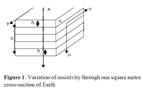
The resistance for a current flowing through the i^th layer of such a column is given by:

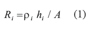
Where, A = 1 m²

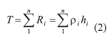
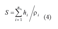
The total transverse resistance through a one square meter column perpendicular to the bedding plane (T) is:

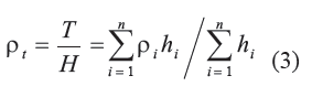
The average transverse resistivity across bedding plane (ρ_t) is:

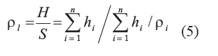
For a current flowing along the bedding planes, the total conductance for the n layers is:

The average longitudinal resistivity for a horizontal current flow is:

The dependence of resistivity on the flow of current is called the coefficient of anisotropy given by the expression;

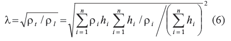
From the derivation of the formula above, it can be deduced that the coefficient of anisotropy depends on the geo-electric section, which may in turn depend on the geologic section (stratigraphic) for rocks covering a long geological period (Groshong, 1997).

According to Kunetz (1966), the coefficient of anisotropy given by equation (6) above, also represents the flattening coefficient for a homogeneous but anisotropic medium where the equipotential surfaces about a point source of current are flattened ellipsoids of revolution.

3. Magnetotelluric prospecting and coefficient of anisotropy

From measurements taken using the magneto-telluric method at the surface, it is possible to identify the anisotropy of the subsurface for the structural trend of a region (Mbom-Abane, 1997). The same author says "close to a lateral heterogeneity, the boundary conditions imposed on the electric field intensity necessitate that the tangential component of the field (E_L) is continuous while the transverse component (E_T) is discontinuous with respect to the resistivity contrast". This implies that ρ_l varies very little, while ρ_t varies tremendously near the heterogeneity. In another manner, Ritz (1982) showed that for a 2-D model made up of two adjacent blocks with quite different apparent resistivities (fault, contact, fracture, and intrusion); the telluric current circulates along the strike of the more resistive block. In such a situation, it is possible to determine the anisotropy given by ρ_t/ρ_l, where according to Telford et al., (1990) ρ_t represents the maximum resistivity while ρ_l represents the minimum.

The ratio ρ_t/ρ_l, can be used in a 2-D structure to locate the boundary between conductive and resistive blocks, and to determine the direction chosen by telluric current near important discontinuities. Furthermore, from a pseudo-section of apparent anisotropy drawn using the variation of λ= √ ρ_t/ ρ_l with the lateral distance, we can be able to distinguish completely isotropic from completely anisotropic zones, and zones of quite different anisotropies. This therefore, enables us to follow the variation of resistivity in the direction of the principal axes. To conclude, the "pseudo-section of anisotropy could be an important tool for an initial modelling". In separate studies, Koziar et al., (1978) and Strangway (1979) constructed diagrams of variation of apparent anisotropy log ρ_t/ρ_l along a profile as a function of frequency. Adam (1996) also used the numerical model with anisotropic basement resistivity to give an explanation to the geologic features in the Pannonian basin in Hungary. All of these show the importance of coefficient of anisotropy in electrical prospecting.

In this work, we shall show, using the equation λ= √ ρ_t/ ρ_l derived above, that the fidelity of the measured values of apparent resistivity and the choice of the principal directions of prospecting could be determined by an on the spot calculation of the values of coefficient of anisotropy; and that the nature of the subsurface in any area where magneto-telluric prospecting is carried out could be determined using the iso-anisotropy contour maps.

4. Presentation of results

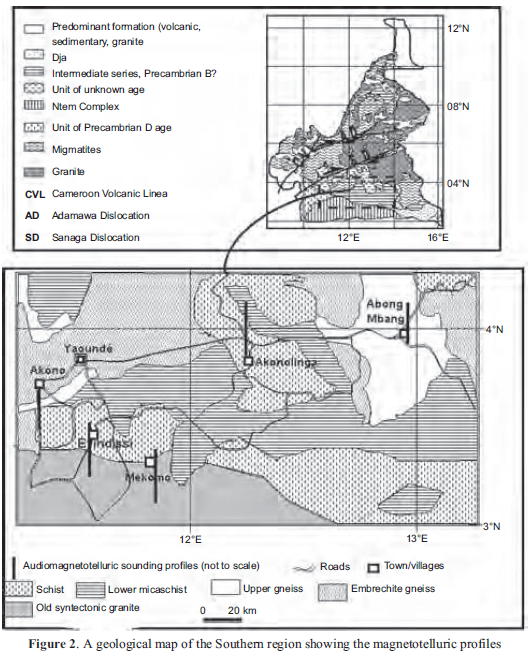
The results presented here were got from audiomagnetotelluric prospecting data on five profiles in two different regions; the Congo Craton and the Pan African Mobile belt (figure 2). The part of the Congo Craton under study is considered in Cameroon as the Ntem complex, which is of the Archean and Proterozoic ages (2900 Ma), represented by a granitic series (Mbom-Abane, 1997). A general feature of the rocks in this region is their schistosity, which shows an external expression of intense metamorphism. This is considered as the seat of the Pan African tectonic events of Central Africa, constituting a major structure of the Pan African orogenesis, which covers a major part of the Cameroonian territory (Bessoles and Lassere, 1977). The Pan African belt is found at the northern edge of the Ntem complex still inside the Cameroonian territory. This region is also the transition zone where the craton formation comes into contact with the Pan African Mobile belt (Njingti-Nfor, 2004)

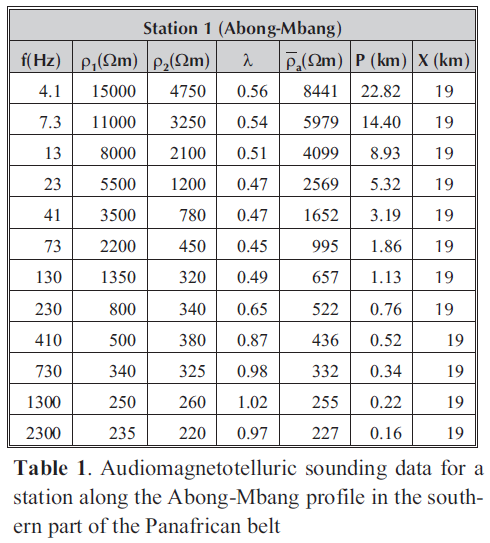
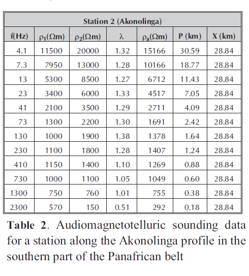
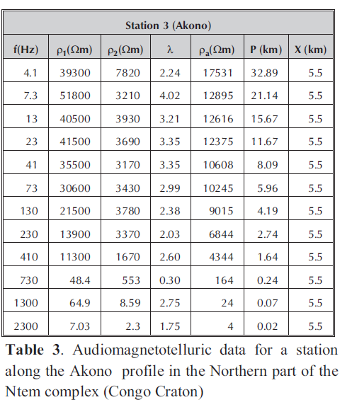
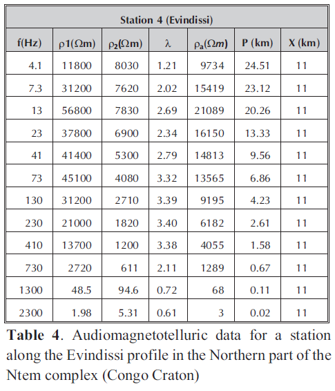
Data for this work were collected firstly between 1986 and 1988 during a detailed audiomag- netotelluric survey of the southern Cameroon by Manguelle-Dicoum (Manguelle-Dicoum et al., 1987) and secondly between 1994 and 1996 by Mbom-Abane and others (Mbom-Abane, 1997). The data were collected at an average of 2 km interval for all Audiomagnetotelluric stations including base stations, on all available roads and tracks in the area, using the ECA resistivimeter (Benderitter et al., 1978; Manguelle-Dicoum et al., 1987) which gives frequency values ranging from 4.1 Hz to 2300 Hz, and automatically calculates and displays the apparent resistivity values for each chosen frequency. We present in tables 1, 2, 3 and 4 sample data of the audiomagnetotelluric sounding for the two regions considered.

Tables 1 and 2 represent results from two stations (Abong-Mbang and Akonolinga profiles) in the Pan African Mobile belt. Table 3 and 4 represent results from two stations (Akono and Evindissi profiles) in the Ntem complex. Each of the tables consists of the frequency of penetration (hertz) in the first column; the longitudinal apparent resistivity values (Ohm-metres) in the second column; the transverse apparent resistivity (Ohm-metres) in the third column; the coefficient of anisotropy in the fourth column; the geometric mean values of apparent resistivity (Ohm-metres) in the fifth column; the depth of penetration (kilometres) in the sixth column and finally the horizontal distance of the station fromthe origin (kilometres) in the seventh column. The coefficient of anisotropy is calculated from the formula (6) derived above. The pseudo-depth of penetration is got from the skin-effect formula (Cagniard, 1953), given by:

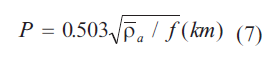
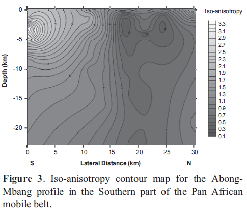
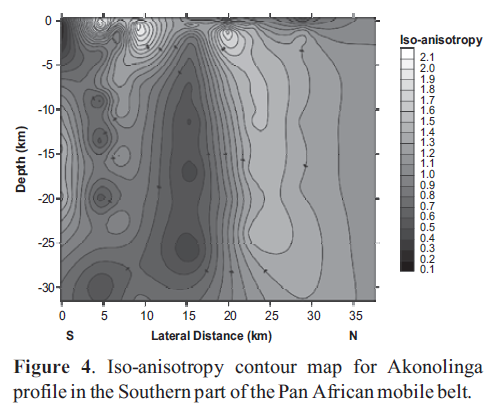
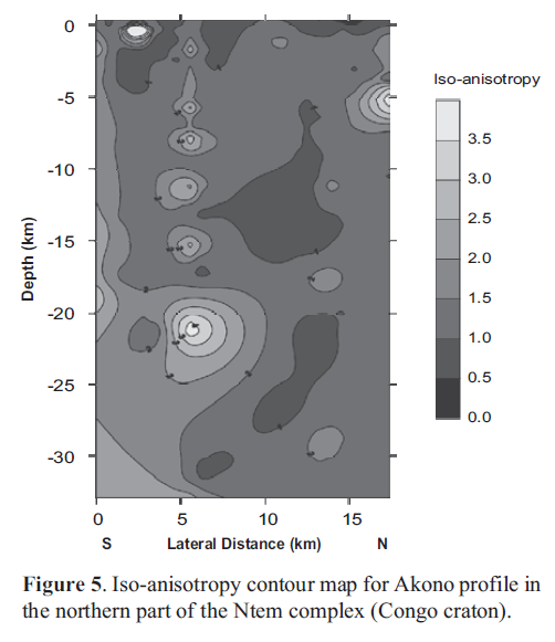
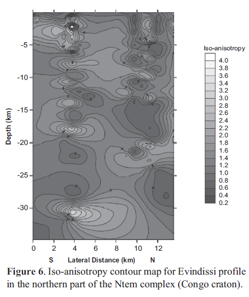
Where, ρ_a is the geometric mean apparent resistivity value in the two principal directions. From these data tables, the iso-anisotropy contour maps presented in figures 3 to 6 are drawn for the five profiles in the two regions. Figures 3 and 4 represent contour maps of Abong-Mbang and Akonolinga profiles respectively located along the 4°N in the southern edge of the Pan African Mobile belt. Figures 5 and 6 represent contour maps of Akono and Evindissi profiles respectively found inside the northern portion of the Ntem complex (Congo craton). Each contourmap has on the vertical axis the pseudo-depth of penetration of telluric current; on the horizontal axis, the lateral separation of stations with one of them chosen as origin, and the plots are the iso-anisotropy contour lines. Each contour line represents an interconnection of points with the same coefficient of anisotropy

5. Interpretation of results

5.1 General discussion

The data from magnetotelluric measurements are usually associated with a number of uncertainties which are related to the limitations of the instrument used, the measured values of apparent resistivity and the various methods of interpretation (Njingti-Nfor, 2004). According to Kunetz (1966), the coefficient for most rocks lies between 1 and 2, although in the same work, he reveals that the coefficient of anisotropy of inter-bedded anhydrite and shale rocks from north eastern Colorado lies between 4.0 and 7.5 for anthracite coal and associated rocks, graphite and slate between 2.0 and 2.8, for inter-bedded limestone and limey shale from north eastern Colorado between 2.0 and 3.0.While using the ratio of maximum to minimum resistivity, Telford et al., (1990) demonstrated that the values of coefficient of anisotropy may be as large as 2 in some graphitic slates, and varies from 1 to 1.2 in rocks such as limestone, shale and rhyolite. Using the square root of the ratio of maximum to minimum resistivity, Njingti-Nfor et al., (2001) calculated the coefficients of anisotropy for various rock types in the Douala sedimentary basin, which had a range of 1.02 to 1.06 for inter-bedded shale and sandstones, massive shale beds and alluvium thick sections.

In this work, our aim is to prove that the coefficients of anisotropy can be a useful tool in determining the principal directions of prospecting and interpreting the data so obtained. Using themagnetotelluricmethod, we have taken a range of coefficients of anisotropy between 0.5 and 2.0, considering the various uncertainties stated above. In the field, the rocks traversed by the telluric current are arranged in the directions of the transverse and longitudinal resistivity values, which are determined on the surface by the method of rotation (Manguelle-Dicoum, 1988). Our considerations presuppose that there is symmetry in the principal directions and that the value 0.5 can be rounded up to 1 so as to tie with Kunetz's proposed range. In a separate study done by drawing profiles of apparent anisotropy for the variation of log(ρ_t/ρ_l) as a function of lateral distance Mbom-Abane (1997), deduced that rocks of low resistivity have negative log values while those of high resistivity have positive log values.

In the present study, it is considered that high resistivity values are in the transverse direction to the line of structure while low resistivity values are along the line of structure as defined on the surface. Coefficients of anisotropy between 0 and 0.5 are considered as those for which the reverse is true and thus, necessitate a change of orientations for the principal directions. Coefficients of anisotropy greater than 2.0 are considered as those due to intrusive bodies such as dykes, sills, batholiths and laccoliths caused by materials welling from below the earth, which will normally have resistivities higher than the host rocks and therefore create an unconformity in resistivity resulting to very high values of coefficient of anisotropy.Faults will also lead to an upset in the layering thus resulting to a change in resistivity variation, which leads to two separate blocks with different coefficients of anisotropy. Fractures create lines of weakness in the layering and result to a break in the resistivity continuity.

5.2 Interpretation of the tables of results

When we look through the data presented in Table 1, from the surface to a depth of 0.76 km, the values of coefficient of anisotropy fall within the range from 0.65 to 1.02; this means that the layers of earth traversed by the telluric current are arranged in the same order as determined on the surface. The values become constant within the range from 0.49 to 0.56; from a depth of 0.76 km right down to a depth of 22.82 km, the layers of the earth traversed by the same telluric current. This arrangement confirms the nature of the station under consideration, which is found around the zone of contact between the Congo craton and the Pan African belt. For table 2, from the surface to a depth of 0.18 to 30.59 km, the coefficient of anisotropy varies from 0.51 to a maximum of 1.38. This variation is in complete conformity with the principal directions determined at the surface. This confirms the nature of the region which although relatively mobile, is considered to have been put in place by radially directed tectonic forces resulting to intrusions within the set-up that became consolidated through contact metamorphism (Badgley, 1965).

Tables 3 and 4 represent data from sample stations that are found right inside the Congo craton. A global look at the three tables shows that the values of the coefficients of anisotropy are within the range of our definitions. However, tables 3 and 4 have values of coefficient of anisotropy which but for a few cases are greater than 2; this therefore indicates that though stable, the subsurface rocks in this region originated from an intense tectonic activity. This activity led to intrusions of undefined magnitudes. This arrangement also shows that the region (craton) has suffered from tectonic movements resulting to intrusive bodies in the architectural set-up.

6. Zonal interpretation

6.1 Interpretation of the iso-anisotropy contour maps

The two regions being considered here are regions where geological and geophysical investigations have already been made. We are going to base our arguments on these early studies in order to interpret the results of the present investigation. A general observation of the contour maps presented from figures 3 to 6 shows that:

•The contour lines are neither completely horizontal nor completely vertical but their shapes are generally distorted and they tend to cluster at some points forming concentric ellipsoids, circles, or cycloids. These shapes depict deformed ellipsoids of revolution, which ties with the description by Kunetz (1966).

• The ellipsoids are separated from each other by sparsely distributed and in most cases deformed contours. These ellipsoids are either concentric around a resistive centre or around a conductive one. This observation ties with the conclusion by Mbom-Abane (1997) according to which the negative values of the log of coefficients of anisotropy represent conductive blocks while the positive values represent the resistive blocks of earth. It should however be noted that talking about resistive and conductive blocks here is just relative because what can be considered a resistive block in a sedimentary region will not be the same as in metamorphic or volcanic regions like the Congo Craton and the Pan African Mobile belt. Knowledge about the region from other investigations is therefore necessary for a conclusion to be drawn.

6.2 The Pan African belt

The Abong-Mbang and the Akonolinga profiles figs. 3 and 4 are both found at the southern edge of the Pan African Mobile belt of Central Africa located between 12°E and 13°30'E each traversing the 4°N parallel right inside the Cameroonian territory. Earlier studies were carried out in this region by Mbom-Abane (1997), using the magnetotelluric prospecting and Tadjou et al. (2004); using gravity method. Their studies showed a general ENE-WSW to E-W structural
trend in Abong-Mbang and a WNW-ESE trend in Akonolinga. These reveal a major deep-seated tectonic dislocation in the whole region with a general W-E direction. Looking at the iso-anisotropy contour map for the Abong-Mbang profile presented in Figure 3, we observe that there are two blocks, on bounded to the South by the 1.4 iso anisotropy contours, and the other to the north by the 0.8 iso-anisotropy contours. Judging from the values of the coefficient of anisotropy, we can conclude that the southerly block is resistive while the northerly block is conductive.

The contour for the Akonolinga profile presented in Figure 4 reveals a conductive block bounded by the 0.7 contour line completely embedded and sandwiched between two resistive blocks bounded by the 1.3 contour line to the South and to the North. If we consider the conductive block as presenting a line of weakness within the subsurface, then each profile has such a line oriented in a West-East direction, thus confirming earlier studies. The limited vertical thickness of the crust suggests that it may be produced by subsidence entirely within the basement, associated with intrusion of low resistive or conductive rocks (granitic intrusion) beneath the region. The extensive form of the iso anisotropy map (Figures 3 and 4) coupled with the consistent nature of gradients along its flanks suggest the presence of two crustal blocks of different mean resistivity and thickness separated by a suture formed by plate collision. This zone marks the boundary of the craton from the Panafrican fold belt.

6.3 The Congo Craton

The Akono and the Evindissi profiles are both found within the Ntem complex, at the northern edge of the Congo Craton located between 11°15'E and 12°E and between 3°N and 3°45'N right inside the Cameroonian territory. Earlier studies in this region were carried out Manguelle-Dicoum (1988) and Manguelle-Dicoum et al., (1992) using the magneto-telluric and by Tadjou (2004) and Tadjou et al., (2004) using the gravity method. In these works, they did not only put into evidence, but also localised a schist-granite metamorphic contact in the area. Their findings are new with respect to the first geological hypothesis according to which the fault and contact in this region matched with each other. From these geophysical data and other geological considerations, these discontinuities are such that one is an intra-granitic basement fracture, while the other is a contact to the north between the schist and the granite. All of these discontinuities have a general W-E direction.

When we look at the iso-anisotropy contour map of the Akono profile as presented in figure 5, we observe a portion of high density contour lines to the South and portion of low density to the North, separated by two portions of sparsely distributed contour lines. Both portions start at the near surface and extend right down the whole depth of the profile. Inside the structure of low anisotropy portions are intrusions of high anisotropy values. The iso-anisotropy contour map of the Evindissi profile as presented in figure 6 shows three portions of sparsely distributed contour lines separated by two high-density portions. One of these portions is to the south, one in the middle and the other to the north of the profile. Unlike the one to the north, which ends mid-way down, the two others start from the surface and extend right down the depth of the profile. There is an interconnection between these portions at various depths, showing that they might have the same origin.

We may conclude that the two major discontinuities in each profile coincide with those put into evidence by Manguelle-Dicoum et al., (1992) and verified by Njingti et al., 2001a and Tadjou et al., (2004) with the southerly located discontinuity representing what was earlier called an intra-granitic discontinuity, while that towards the north represent the schist-granite contact. These contacts represent a major tectonic dislocation in the region. The northern contact (Akonolinga-Abong Mbang zone) may represent a major discontinuity, which can be related to the transition between the Congo craton to the South and the Pan African mobile belt to the North.

Interpretation presented in Figures 3 to 6 supposes that the structures of the region, which are consist of low density schistose rocks (Manguelle-Dicoum et al., 1992; Tadjou et al., 2004), were put in place beneath the surface by a combination of subsurface subsidence and piecemeal stopping. The intrusion presumably represents a magma chamber, with high-resistive materials. The role played by this area during the Pan African episode is recorded at the surface by outcrops of granites in the south, and by plutonic rocks (granulites) within the fracture zone in the north.

We have shown in this work that an on the spot calculation of coefficients of anisotropy can in addition to the method of rotation be a very useful way of determining the direction of structural trend of the geologic features in a particular region of prospecting. This is because, from the calculated values of coefficient of anisotropy, which should lie between 1 and 2 (Kunetz, 1966) or between 0.5 and 2.0 as stated in this work, it is possible to know the way the various layers traversed by the telluric current are oriented as a function of the frequency or depth of penetration. Any value below 1 shows a change in the orientation of the layers or bedding planes since the coefficient of anisotropy is the square root of the ratio of the transverse apparent resistivity to the longitudinal. Any value greater than 2 represents an unconformity in coefficient of anisotropy, which could be caused by an intrusion of a body of exceptionally high resistivity, a fracture which results to a break in conductivity continuity, faults, or any other structure that cuts vertically through the directional trend of the structure. Lengthening the telluric line will increase the value of the coefficient of anisotropy if the lateral spread of the intrusive structure is more in one direction than the other. Thus in the field, by manipulating on the telluric line, we can identify the structure in question.

We have succeeded in this work in showing that iso-anisotropy contour maps provide a more effective and efficient representation of the variation of apparent resistivity with depth for a vertical cross-section through a slice of Earth under consideration. The different structures form by the tectonic movements within the earth such as faults, folds, and intrusions, their types and manifestations have been clearly depicted on the contour maps with high lateral gradients. This thus enables us to identify structures like contacts, dykes, fractures and faults. The various forces responsible for the formation of these structures, their nature and directions have been revealed through the shapes of the contour lines. The whole vertical cross-sectional architectural framework for a given profile has been highlighted. It has also been shown that from the values of anisotropy we can have an idea of the rocks formation in the region of investigation. For example, we have seen that, sedimentary regions are less deformed and therefore have values of coefficient of anisotropy that may fall strictly within the defined interval. On the other hand, metamorphic regions suffer from a lot of tectonic and oscillatory movements leading to conformed and unconformed layering, with values of anisotropy not only lying within but also beyond the defined interval. It therefore means that this method could be used as a reconnaissance for a region where the researcher has a poor knowledge of its geology.

1. Adam, A. 1996. Regional magnetotelluric anisotropy in the Pannonian basin (Hungary). Acta Geod. Geoph. Hung., vol. 31(1-2), pp. 191-215.        [ Links ]

2. Bessoles, B., Lasserre, M. 1977. Le complexe de base du Cameroun. Bull. Soc. Geol., France, t XIX, No 5, pp. 1085-1092.        [ Links ]

3. Badgley, P. C. 1965. Structural and tectonic principles:Harper & Row LTD, New York.        [ Links ]

4. Benderritter, Y., Herisson, C., Korhenen, H., and Pernu, T. 1978. MTexperiments in Northern Finland. Geophysical prospecting, 26, 562-571.        [ Links ]

5. Cagniard, L. 1953. Principe de la méthode magnétotellurique, nouvelle méthode de prospection géophysique. Ann. de géophysique, t.9, fasc.2, 95-125.        [ Links ]

6. Frischknecht, F.C., Keller, G. V. 1966. Electrical methods in applied geophysics. London, Pergamon.        [ Links ]

7. Groshong, R.H. Jr .1997. 3D structural Geology. A guide to structure and surface map interpretation. Springer, Verlag Berlin; Heidelberg New-York.        [ Links ]

8. Koziar A., Strangway, D. W. 1978. Shallow crustal sounding in the Superior Province by A. M. T. Can. J. Earth Sc., 15, 1701 – 1711.        [ Links ]

9. Kunetz, G. 1966. Processing and interpretation of magnetotelluric soundings. Geophysics 37, 1000-1021.        [ Links ]

10. Manguelle-Dicoum, E., Bokosah, A. S., Kwende-Mbanwi, T. E. 1987. Détermination des directions principales de structure de la faille de Mbalmayo. Ann. Fac. Sci. Terre IV(3-4), 149-171.        [ Links ]

11. Manguelle-Dicoum, E. 1988. Etude Géophysique des structures superficielles et profondes de la région de Mbalmayo. Thése de Doctorat es-sciences (Géophysique). Université de Yaoundé, 202 pages.        [ Links ]

12. Manguelle-Dicoum, E., Bokosah, A. S., Kwende-Mbanwi, T. E. 1992. Geophysical evidence of a major Precambrian schist-granite boundary in Southern Cameroon. Tectonophysics, 205, 437-446.        [ Links ]

13. Mbom-Abane, S. 1997. Investigations géophysiques en bordure du Craton du Congo et implications structurales. Thése de Doctorat és Sciences. Université de Yaoundé (Cameroun), 180p.        [ Links ]

14. Njingti-Nfor, Manguelle-Dicoum, E., Mbom-Abane, S., Tadjou, J. M. 2001a. Evidence of major tectonic dislocations along the southern edge of the Pan African mobile zone and the Congo craton contact in Southern region of Cameroon. Proceedings of the Second International Conference on the Geology of Africa, Assiut, Egypt, Vol. (I), pp. 799-811.        [ Links ]

15. Njingti-Nfor, Manguelle-Dicoum, E., Tabod, C.T., Tadjou, J. M. 2001b. Application of audiomagnetotellurics soundings to determine the types of rocks and their geologic ages. (A case study of the eastern edge of the Douala sedimentary basin in Cameroon). Proceedings of the Second International Conference on the geology of Africa, Assiut, Egypt, Vol. (I), pp.787-797.        [ Links ]

16. Njingti-Nfor, 2004. New methods of analysing and interpreting audiomagnetotelluric data. de Doctorate thesis, Univ. Yaoundé I, 185 pages.         [ Links ]

17. Postma, G. W. 1955. Wave propagation in a stratified medium. Geophysics, 20, 780-806.        [ Links ]

18. Ritz, M. 1982. Etude regionale MT des structures de la conductivité électrique sur la bordure occidentale du Craton Ouest Africain en République du Senegal. CAN. J. Earth Sci., 19, 1408-1416.        [ Links ]

19. Strangway, D.W., Koziar, A. 1979. AMT sounding-A case history at the Cavendish geophysical test range. Geophysics, 44 (8), 1429-1446.        [ Links ]

20. Tadjou, J. M., 2004. Apport de la gravimétrie à l’investigation géophysique de la bordure septentrionale de Craton du Congo (Sud-Cameroun). Thése de Doctorat/Ph.D, Univ. Yaoundé I, 178 pages.        [ Links ]

21. Tadjou, J.M., Manguelle-Dicoum, E., Tabod, C.T., Kamguia, J., Nouayou, R., Njandjock, N. P., Ndougsa-Mbarga, T. 2004. Gravity modelling along the northern margin of the Congo craton, South Cameroon. Journal of the Cameroon Academy of Sciences, 4(1), 51-60.        [ Links ]

22. Telford, W. M., Geldart, L. P., Sheriff, R. E., Keys, D. A. 1990. Applied Geophysics. Cambridge University Press.        [ Links ]

23. Uhrig, L. F. and Van-Melle, F. A. 1955. Velocity anisotropy in stratified media: Geophysics, 20, 774-779.        [ Links ]

24. Vozoff, K. 1990. Magnetotelluric: Principle and practice. Proc. Indian Acad. Sc. (Earth Planet.Sci.), vol. 99(4), 441-471.         [ Links ]