Thin-layer detection using spectral inversion and a genetic algorithm

Kelyn Paola Castaño¹, Germán Ojeda² and Luis Montes¹

¹ Universidad Nacional de Colombia, Facultad de Ciencias, Departamento de Geociencias, Sede Bogotá, Colombia. E-mail: kpcastanog@unal.edu.co, lamontesv@unal.edu.co

² ECOPETROL S.A. Bogotá, Colombia. E-mail: g.ojeda@ecopetrol.com.co

Record

manuscript received: 30/04/2011 Accepted for publications: 10/12/2011

ABSTRACT

Spectral inversion using a genetic algorithm (Ga) as an optimisation approach was used for increasing the seismic resolution of a particular dataset; by contrast with the conjugate gradient method, a Ga does not require a good starting model but rather a search space.

The method discriminated layers thinner than λ/8 when tested on synthetic and log data. When applied to a seismic dataset concerning the Barco formation in the Catatumbo basin, Colombia, spectral inversion led to recovering information from seismic data contributing towards the vertical identification of geological features such as thin distributary channels deposited in a deltaic environment having a tidal influence. The results revealed that a GA outperformed traditional minimisation schemes.

Keywords: genetic algorithm, spectral inversion, seismic inversion, Barco formation, Catatumbo basin, seismic resolution.

RESUMEN

La inversión espectral, a partir de un algoritmo genético fue usado como estrategia de optimización, e incremento de la resolución de un volumen sísmico. Contrario al método del gradiente conjugado, el algoritmo genético no requiere un buen modelo inicial sino un espacio de búsqueda.

Usado en datos sintéticos y registros de pozo el método discriminó capas tan delgadas como A/8. Al usarse en un volumen de la formación Barco en la Cuenca del Catatumbo, Colombia, la inversión espectral recuperó información que contribuyó a la identificación de delgados canales distributarios depositados en un ambiente transicional con influencia de mareas. El resultado mostró que esta estrategia es más eficiente y efectiva que los procedimientos convencionales de minimización.

Palabras claves: algoritmos genetico, inversion spectral, inversion sismica, formacion barco, Cuenca Catatumbo, resolucion sísmica.

Introduction

The reliable estimation of thickness during exploration activities can help to delineate prospects despite a lack of well information; it may help in obtaining more accurate volumetric hydrocarbon production calculations and in planning drilling involving lower risk.

Vertical seismic resolution is the key to extracting detailed stratigraphy which can distinguish two close seismic events associated with geological events. Important oil reservoirs often have layers having a thickness which is below seismic resolution. The transitional Palaeocene Barco formation in the Catatumbo Basin consists of varying thickness sand wedges and, as it has several producing oil fields, there is great interest in mapping thin layers within it for drilling future wells. According to the Rayleigh criterion, layers thinner than /8 cannot be resolved by seismic imaging (Kallweit and Wood, 1982; Widess, 1973); tuning-thickness analysis based on this model has been used as a thickness mapping method for several decades now.

Amplitude and frequency variations through layers having changing thickness was used as a tool for extracting stratigraphic details (Partyka et al., 1999), spectral decomposition using discrete Fourier transform (DFT)

The method was tested on synthetic and log data and applied to seismic data for interpreting thin distributary channels deposited in a deltaic environment having a tidal influence.

Geological setting

The Barco formation consists of interbedded fine-grained sandstone with mudstone; it was deposited in a deltaic environment having a tidal influence (Nuñez and Saavedra, 2006). Thin sequences of bioturbated fine-grained sandstone are cross bedded with fine-grained sandstone and gray mudstone. Some coal horizons are present, mainly at the top of this unit. The formation's thickness varies from 500 feet to 700 feet, running northeast to southeast of the basin.

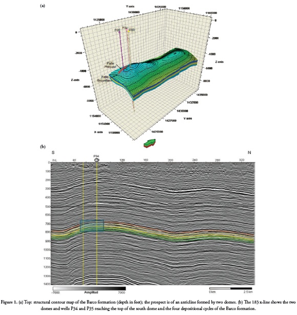
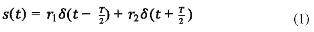
Two folds have been interpreted in the area (Ojeda et al., 2009); a syncline has been located in the western part by the 3D seismic programme, followed by an anticline structure in the eastern part consisting of two domes. A main fault and secondary fault to the east of the former separate these two domes' structures (Figure 1A). Wells P33, P34 and P35 reach the top of the Barco formation on the south dome. This formation is divided into four depositional cycles, each representing a maximum flooding surface and hence stratigraphic limits. Figure 1B shows x-line 183 where the Barco formation and the four depositional cycles link wells P34 and P35.

Theory

An appropriate seismic attribute must be directly sensitive to geological features or reservoir properties, allowing a geologist to interpret a geological structure and its particular environment. Coherence integrates information contained in adjacent traces to extract information which may not be easily recognised on time scale maps; high coherence thus indicates lateral lithological continuity whereas abrupt changes may suggest faults and fractures (Chopra & Marfurt, 2007). Fault-to-fault coherence is used to enhance stratigraphic and structural discontinuity, discerning faults and channel geometry. Root mean square (RMS) amplitude may be applied to recognise seismic anomalies and squaring amplitude values within an analysis window can enhance important amplitudes above noise level. On other hand, combination of attributes has been used to characterize reservoirs (Guerrero et al, 2010) and has allowed identify channels in transitional environment with tidal influence.

Spectral inversion

Due to the Widess model occurring in nature as the exception not the rule, spectral inversion is based on the fact that an impulse pair of reflectors can be decomposed in odd and even parts (Castagna, 2004; Chopra et al., 2006). Seismic resolution is increased because the odd part constructively interferes when thickness becomes thinner.

The process differs from conventional methods because inversion is driven by geological knowledge and is based on local frequency spectrum characteristics obtained from spectral decomposition techniques (Marfurt and Kirlin, 2001).

Inversion is defined in this method (Puryear and Castagna, 2008) through an amplitude spectrum's constant periodicity for a layer of given thickness; it takes advantage of the fact that spacing between spectral peaks and notches is precisely the inverse of layer thickness in the time domain (Partyka et al., 1999).

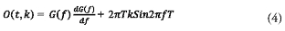
When an analysis point lies at the centre of a layer (in the time domain), the impulse pair may be expressed by:

Here, and are the top and base reflection coefficients and T is layer thickness.

The equation's Fourier transform gives the real and imaginary parts:

where f is frequency, r and r are the odd and even component of the coefficient pair.

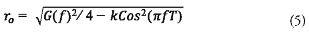
As demonstrated by Puryear and Castagna (2008) there is a cost function O(t,k) given by:

where G(f) is amplitude regarding frequency and Equation 4 is solvable after evaluating O(t, k) at each frequency and finding the global minimum in a k-Tmodel space. r is determined by

and r from .Time sample at t₁ top of reflector r₁ is given

by

g(f) is the complex spectrum for the reflection coefficient pair. Extended to multiple layers and assuming seismograms to be the convolution between r(t) and a known wavelet w(t), the spectral decomposition of a seismic trace s(t) within time window length tw can be expressed as:

A too short window affects frequency resolution and a too long window deteriorates time resolution. When the wavelet spectrum is known, r(t) and T(t) are estimated by optimising the function:

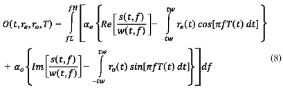
Here, f_Hand f_Lare high cut-off and low cut-off frequency, a_eand a_o are weighting functions. The a /a ratio is adjusted according an acceptable trade-off between noise and resolution and a >> a in the case of the Widess model.

The best solution is achieved when objective function O (t, r, r, T), given by equation (6), is minimised over the frequency rank, supplying model parameters r, r_oand T.

Genetic algorithm

Unlike local optimisation approaches, overall ones attempt to find the misfit function's global minimum, most of them being stochastic by nature. Regarding real data, it can never be known whether an achieved solution is the optimal one; however, even starting with poor initial data, achieved solutions give good results.A genetic algorithm (GA) is widely used in numerical analysis to find accurate solutions for optimising problems because it is one of the best ways to solve a problem about which little is known, thereby creating a relatively quick high-quality solution to a particular problem. A GA tends to thrive in an environment where there are many solutions and in which the search space is uneven and has many hills and valleys. A GA is based on analogies regarding biological evolution (simulated evolution). It uses a population of abstract representations (genome / genotype) of candidate solutions (phenotypes) resolving an optimisation problem. It starts from a randomly-generated population of individuals evolving through successive generations. Each individual's fit in a particular population is evaluated; multiple individuals are stochastically selected (based on their fit) and modified (recombined and randomly mutated) to form a new population. The new population is then used for the algorithm's next iteration. The algorithm usually ends with the maximum number of iterations (generations) or satisfactory adjustment of the target population has been achieved. A GA review is beyond the scope of this document but one treatise is recommended (Glover at al., 2003. Chapter 3, pp55)

Method

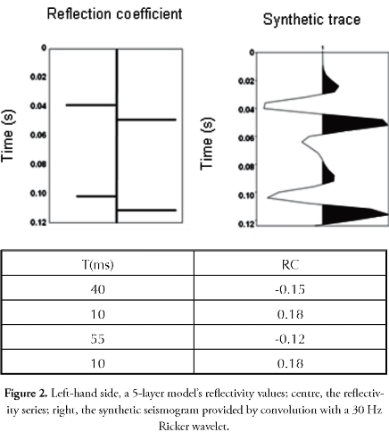
Spectral inversion was first tested on a semi-infinite five-layer model (Figure 2, left-hand side) where a 4 ms sample rate synthetic seismogram was produced by convolving the model's reflectivity series with a 30 Hz Ricker wavelet (Figure 2, right-hand side). The method involved using a 128 ms window centred at 64 ms and applying a 128 m Gaussian-tapered Fourier transform. It was assumed that a = a , i.e. an equal even/odd contribution to the reflection coefficient pair.

The selected seismic data covered a 1 km²-area sub-volume from a post-stacked 3D data survey of the Catatumbo basin containing 1,271 traces. The dataset regarding the top and the bottom of the Barco formation was located at the top of the south dome field concerning an oil producing area considered to be stratigraphically complex. Good quality borehole data regarding the field was available. Data volume was retro-deformed to flatten the top of the Barco formation to avoid structural strain effects appearing in the trace due to trace inversion.

Seismic data quality and vertical seismic resolution were assessed to establish interpretation scope during the initial stage. A 71 m wavelength having 18 m vertical resolution was provided at 40 Hz dominant volume frequency together with 2,850 m/s average speed estimated by sonic logs.

Discussion of results

Synthetic model

Figure 3 shows the cost function pattern calculated for a couple of layers where inversion-estimated values were close to optimum values, having lower than 6 ms estimation errors.

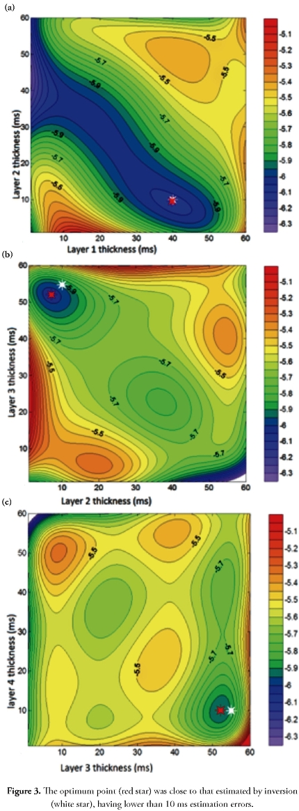
An additional minimum may be observed at the top left of Figure 3A where layer 1 thickness varied from 30 to 60 ms and layer 2 was thinner than 5 ms. Figures 3B and 3C contain other minimums where layer 3 thickness vanished; therefore, the layers had to be constrained to non-zero thickness to avoid such border effect.

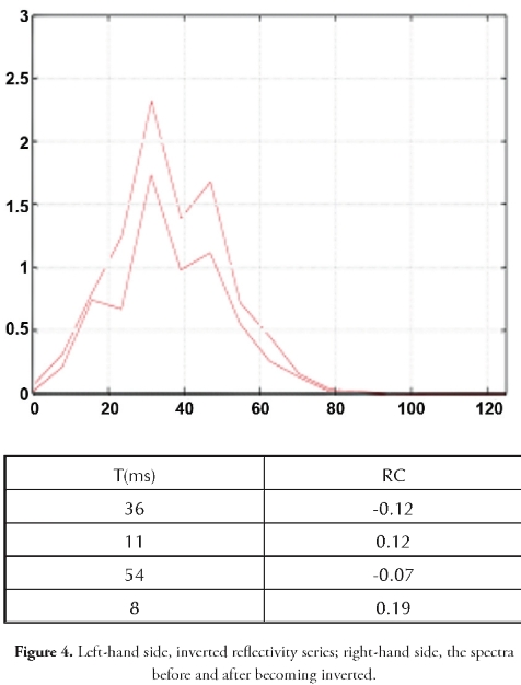
The synthetic seismogram in Figure 2 provided an accurate model when it was inverted, considering the 2 ms seismic resolution and the tiny difference between the expected and obtained reflection coefficients. The foregoing was reinforced by comparing the data's spectra amplitude before and after inversion, depicting a similar pattern and small power decay (Figure 4).

By contrast with the conjugate gradient optimisation method tested by Puryear and Castagna (2008), a GA does not require a good starting model and only needs a defined search space containing a particular solution. A conjugated gradient matrix can be analytically formulated, leading to rapid numerical evaluation; the cost of computing its derivatives makes a GA a faster alternative. A GA introduced performance improvement here by doing a fast exhaustive search and finding a good solution quickly.

Real data

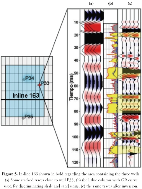
GA was used with spectral inversion with regarding the sub-volume having 1,271 seismic traces and 128 ms window length. The stacked time section was tied to the well and the stacked traces in the volume were inverted. Figure 5 shows stacked traces near the well before (Figure 5a) and after inversion (Figure 5c) and the stratigraphic column (Figure 5b) with the tied reflectors associated with sand (yellow) and shale (grey) packages interpreted from well logs. The inverted reflectors discriminated the top and bottom of sand units whereas the reflectors in original data were associated with the thicker layers having a 10 ms uncertainty time position. Spectral inversion increased vertical resolution discriminating layers within the predicted resolution limit (6 ms) and a well-defined sand-shale sequence was thus determined. The inversion did not recover the top of the sand package at the bottom of the section, probably due to a border effect regarding the restricted window.

Stacked in-line 63 is shown in Figure 6, before (top) and after inversion (bottom), including time resolution and the number of reflectors having lateral continuity. Some discontinuous reflectors in the inverted section's left zoomed-in box, shown by an arrow around 50 ms, suggested an aggradational stack of layers inside a channel which was not visible before inversion. The reflector's geometrical pattern inside the right-hand zoomed-in box suggested the base of a channel around 60 ms; two fluvial seismic patters were observed in the 47 ms time-slice shown later on in Figure 7.

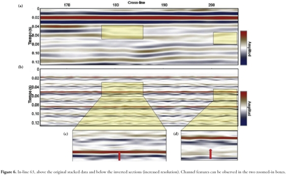
Inverted seismic images revealed vertical detail comparable with well information sharply contrasting with the horizontal seismic resolution imposed by the original acquisition; the 20 ms in-line and the 40 ms x-line separations were not modified by the inversion.

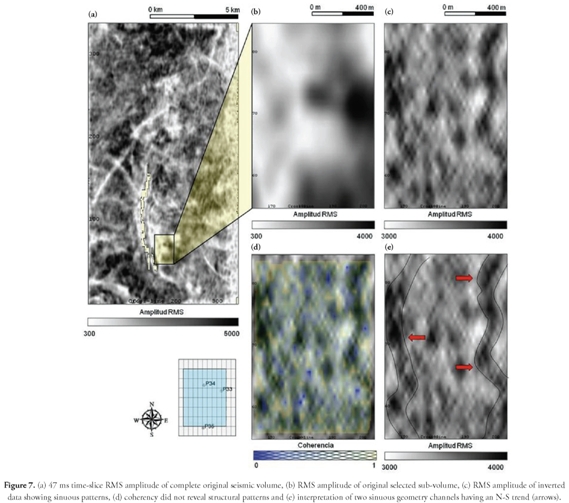
RMS amplitude and seismic volume coherence were calculated before and after inversion. The RMS amplitude 47 ms time-slice is shown in Figure 7a, a box limiting the zoomed-in area. RMS amplitude 17 ms time-slice and inverted data coherence are shown in Figures 7b and 7c, respectively, where the RMS image shows an N-S sinuous continuity pattern to the east, interpreted as being a small meandering distributary channel which was consistent with the ICP palaeoenvironmental interpretation (2006) and supported by core analysis of well P33 drilled in the channel. Another sinuous pattern observed to the west was interpreted as a meandering channel; by contrast, these patterns were not observed in RMS amplitude before inversion (Figure 7b), probably due to the tuning thickness effect.

17 ms time-slice coherence (Figure 7d) did not reveal structural seismic patterns as being faults or dipping reflectors, thereby agreeing with the absence of important structures in the sub-volume.

Increased horizontal resolution would lead to facies identification supporting the above interpretation; however, there were artefacts and noise levels revealing limitations in horizontal resolution which were related to bin size and footprint effect.

Conclusions

Thickness constraints in spectral inversion should be used as input for more accurate model-based reflectivity inversion. A GA minimisation algorithm performed well, achieving greater accuracy and faster execution.

Thickness inversion from real data clearly showed layering below seismic resolution and above 6 ms, i.e. our data's predicted resolution limit. Inversion, however, failed to capture the top of a sand package at the bottom of the section, suggesting that there was a border effect in the analysis window.

Lower than seismic resolution sand and shale packages can be resolved through spectral inversion and correlating them with stratigraphic information derived from well logs. The inversion method had the necessary power for resolving the vertical top and bottom reflectors associated with thin layers.

RMS amplitude of inverted data indicated meandering sinuous geometries which were possibly related to small distributary channels on a tidal plain. However, horizontal resolution should be improved to identify facies association thereby leading to a conclusive result.

Time-slice coherency did not reveal any evidence related to structural features, this being consistent with the absence of important structures in the selected sub-volume.

This methodology has provided information making a significant contribution to the vertical identification of geological features such as thin distributary channels in a flat tidal environment. However, it is recommended that future studies should be carried out aimed at solving problems related to seismic horizontal resolution.

Acknowledgements

The authors would like to thank William Agudelo, Carlos Piedrahita and Jorge Monsegny from the Instituto Colombiano del Petróleo (ICP) for their support and contributions and also Dr. Jonh Castagna for discussion regarding the concepts behind spectral inversion. Financial support and data permission was provided by ECOPETROL S.A. This paper has resulted from an MSc thesis in Geophysics written by Kelyn Castaño at the Universidad Nacional de Colombia.

References

Castagna, J. P. (2004). Spectral decomposition and high resolution reflectivity inversion. Ann. SEG Meeting, Tulsa, Oklahoma.        [ Links ]

Chopra, S., Castagna, J. P., and Portniaguine, O. (2006). Seismic resolution and thin-bed reflectivity inversion. Canadian Society of Exploration Geophysicists Recorder, 19—25.        [ Links ]

Chopra, S., and Marfurt, K. J. (2007). Seismic attributes for prospect identification and reservoir characterization. (S. J. Hill, Ed.) Tulsa, Oklahoma, USA: SEG - EAGE.        [ Links ]

Glover F. and Kochenberger G., (2003). Handbook of Metaheuristics. International series in operational research and management series. International Academic Publishers. Norwell, Mass. Chapter 3. Genetic Algorithms. Pp. 55-82.        [ Links ]

Guerrero J., Vargas, C. and Montes, L. (2010). Reservoir characterization by multiattribute analysis: The Orito field case. Earth Sci. Res. J. (14), 173-180.        [ Links ]

Kallweit, R. S., and Wood, L. C. (1982). The limits of resolution of zerophase. Geophysics (47), 1035—1046.        [ Links ]

ICP. (2006). Evaluación integrada de yacimientos campos área Lisama, área Llanito y Sardinata. Santander. Piedecuesta: ECOPETROL S.A.        [ Links ]

Nuñez, M., y Saavedra, J. L. (2006). Definición de un modelo estático para las formaciones Barco y Catatumbo, Campo Sardinata, Cuenca Catatumbo, Colombia. Bucaramanga: Universidad Industrial de Santander, Facultad de Ingenierías Fisicoquímicas, Escuela de Geología.        [ Links ]

Marfurt, K. J., and Kirlin, R. L. (2001). Narrow-band spectral analysis and thin-bed tuning. Geophysics, 66 (4), 1274—1283.        [ Links ]

Ojeda, G. Y., García, P. A., Rubiano, J. L., and Gómez, F. H. (2009). Multi-attribute-based net sand estimation in transitional reservoirs: Barco formation, Sardinata Field, Colombia. SEG Expanded Abstracts, 3530-3533.        [ Links ]

Partyka, G. A., Gridley, J. A., and López, J. A. (1999). Interpretational aspects of spectral decomposition in reservoir characterization. The Leading Edge (18), 353-360.        [ Links ]

Partyka, G. A. (2005). Spectral decomposition: SEG Distinguished Lecture. (SEG, Editor) http://ce.seg.org/dl/spring2005/partykaabstract.shtml (2006).        [ Links ]

Peyton, L. R., Bottjer, R., and Partyka, G. (1998). Interpretation of incised valleys using new 3D seismic techniques: A case history using spectral decomposition and coherency. The Leading Edge (17), 1294-1298.        [ Links ]

Portniaguine, O., and Castagna, J. P. (2004). Inverse spectral decomposition. 74^th Annual International Meeting,SEG, Expanded Abstracts, 1786-1789.        [ Links ]

Puryear, C. I., and Castagna, J. P. (2008). Layer-thickness determination and stratigraphic interpretation using spectral inversion: Theory and application. Geophysics, 73 (2), 37-48.        [ Links ]

Sen, M., and Stoffa, P. L. (1992). Multilayer AVO inversion using genetic algorithms. Proceedings of the SEG/EAEG Summer Research Workshop (6), 581-589.        [ Links ]

Widess, M. B. (1973). How thin is a thin bed? Geophysics, 38 (6), 1176-1180.        [ Links ]