Reference crust-mantle density contrast beneath Antarctica based on the Vening Meinesz-Moritz isostatic inverse problem and CRUST2.0 seismic model

Robert Tenzer¹ and Mohammad Bagherbandi^2,3.

¹Institute of Geodesy and Geophysics, School of Geodesy and Geomatics, Wuhan University, 129 Luoyu Road, Wuhan, China

²Division of Geodesy and Geoinformatics, Royal Institute of Technology (KTH), SE-10044 Stockholm, Sweden

³Department of Industrial Development, IT and Land Management University of Gävle, SE-80176 Gävle, Sweden

Recibido: 23/10/2012 - Aceptado: 04/04/2013

ABSTRACT

The crust-mantle (Moho) density contrast beneath Antarctica was estimated based on solving the Vening Meinesz-Moritz isostatic problem and using constraining information from a seismic global crustal model (CRUST2.0). The solution was found by applying a least-squares adjustment by elements method. Global geopotential model (GOCO02S), global topographic/bathymetric model (DTM2006.0), ice-thickness data for Antarctica (assembled by the BEDMAP project) and global crustal model (CRUST2.0) were used for computing isostatic gravity anomalies. Since CRUST2.0 data for crustal structures under Antarctica are not accurate (due to a lack of seismic data in this part of the world), Moho density contrast was determined relative to a reference homogenous crustal model having 2,670 kg/m³ constant density. Estimated values of Moho density contrast were between 160 and 682 kg/m³. The spatial distribution of Moho density contrast resembled major features of the Antarctic’s continental and surrounding oceanic tectonic plate configuration; maxima exceeding 500 kg/m³ were found throughout the central part of East Antarctica, with an extension beneath the Transantarctic mountain range. Moho density contrast in West Antarctica decreased to 400-500 kg/m³, except for local maxima up to ≈ 550 kg/m³ in the central Antarctic Peninsula.

Key words: Antarctica, crust, gravity, isostasy, mantle, Moho interface.

RESUMEN

El contraste de densidad de la discontinuidad de Mohorovicic (Moho) debajo de la Antártida fue estimado con base en la solución del problema isostático Vening Meinesz-Moritz y a partir de datos obtenidos con el modelo sísmico de la corteza global (CRUST2.0). La solución se encontró a través de un ajuste al método de mínimos cuadrados por el método de elementos. El modelo geopotencial global (GOCO02S), el modelo topográfico/batimétrico (DTM2006.0), los datos de espesor del hielo para la Antártida (reunidos por el proyecto BEDMAP) y el modelo sísmico de corteza global (CRUST2.0) fueron utilizados para calcular las anomalías gravitatorias isostáticas. Ya que los datos de CRUST2.0 para las estructuras de la corteza en la Antártida no son exactos (debido a la falta de información sísmica para esta parte del planeta), el contraste de densidad de la Discontinuidad de Mohorovicic fue determinado a partir de un modelo de corteza homogéneo que tiene una densidad constante de 2,670 kg/m³. Los valores estimados del contraste de densidad de la Moho se encontraron entre 160 y 682kg/m³. La distribución espacial del contraste de densidad de la Moho exhibe mayores rasgos en la configuración de la plancha tectónica de la Antártida continental y su alrededor oceánico. El valor máximo encontrado excede los 500 kg/m³ y se ubica en la parte Este continental, con extensión en las Montañas Transantárticas. El contraste de densidad de la Moho (zona de transición entre la corteza y el manto terrestre) en el Oeste de la Antártida osciló entre 400-500 kg/m³, excepto para la máxima local de ≈ 550 kg/m³, en el centro de la Península Antártida.

Palabras clave: Antártida, corteza terrestre, manto terrestre, gravedad, isostasia, Discontinuidad de Mohorovicic.

Introduction

Current knowledge about the lithospheric structure beneath Antarctica is limited due to a low spatial coverage of high-quality seismic data. Seismic studies by Kogan (1972) and Ito and Ikami (1986) were based on localised controlled source seismic experiments. Passive seismic studies, based on earthquakes occurring mostly outside the Antarctic tectonic plate (due to a lack of intra-plate seismicity within the Antarctic plate (Okal, 1981), still represent the primary source of information. Studies based on an analysis of surface wave velocity can be found in Evison et al., (1960), Kovach and Press (1961), Bentley and Ostenso (1962), Dewart and Toksoz (1965), Adams (1971), Knopoff and Vane (1978), Rouland et al., (1985), Forsyth et al., (1987), Roult et al., (1994) and Bannister et al., (2003). Seismic receiver function analysis has been carried out by Reading (2006), Lawrence et al., (2006) and Winberry and Anandakrishnan (2004). Ritzwoller et al., (2001) used the simultaneous inversion of broadband group velocity measurements to compile a seismic model of the crust and upper mantle beneath Antarctica and surrounding oceans. Some studies have been based on airborne gravity surveys, for instance by Studinger et al., (2004, 2006). Llubes et al., (2003) used CHAMP satellite gravity data for estimating crust thickness in Antarctica. More recently, Block et al., (2009) have estimated crust thickness in Antarctica using GRACE gravity data.

Despite some authors having investigated Antarctic crust thickness, studies addressing lithosphere density structure and density interface in this part of the world are rare. This study was thus aimed at investigating Moho density contrast beneath Antarctic continental and surrounding oceanic crustal structures. Since large areas of Antarctica are not yet sufficiently covered by seismic surveys, current knowledge about crust density structure is not complete and accurate. A simple model of 2,670 kg/m³ homogenous crust reference density was thus adopted and Moho density contrast was estimated regarding such crustal density. This involved applying the method recently developed by Sjöberg (2009) and Sjöberg and Bagherbandi (2011).

Isostatic model

The generic expression of solving the Vening Meinesz-Moritz isostatic problem was formulated in the following form (Sjöberg and Bagherbandi, 2011):

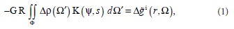
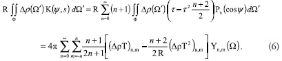
where G = 6.674×10^-11 m³ kg^-1 s^-2 is Newton's gravitational constant, R = 6371×10³ m Earth's mean radius, Δp Moho density contrast, Δg^I (approximate) isostatic gravity anomaly (cf. Sjöberg, 2009), K the integral kernel function, and dΩ'=cosø'dødλ the infinitesimal surface element on the unit sphere. The 3-D position was defined in the spherical coordinates system (r, Ω) where r is the spherical radius and Ω=(ø , λ)denotes the spherical direction with spherical latitude ø and longitude λ. The full spatial angle is denoted as Φ={Ω'=(ø',λ'):ØE[-π/2,π/2]λ'E[2,2π]} . Integral kernel K in equation (1) was defined for parameters Ψ and s, where &Psi is the spherical distance between observation and (running) integration points (r, Ω) and (r', Ω') and s a ratio function of the Moho depth T and Earth's mean radius R, i.e.s=1-t=1-T/R The spectral representation of K was given by (Sjöberg, 2009):

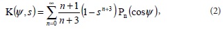
where nP is the Legendre polynomial of degree n for the argument of cosine of the spherical distance . The isostatic gravity anomaly Δg^I computed at position(r, Ω)was defined as follows (cf. Vening Meinesz, 1931):

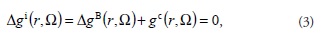
where Δg^B is the refined Bouguer gravity anomaly, and g^c the gravitational attraction of isostatic compensation masses (see also Bjerhammar, 1962, Chap. 14, eqn. 5; Moritz, 1990). The spectral representation of isostatic gravity anomaly Δgⁱ was defined in terms of spherical harmonics Δgⁱ_n,m of degree n and order m. The numerical coefficients Δgⁱ_n,m were generated from spherical harmonic coefficients of gravity anomaly Δgⁱ_n,m after applying the Bouguer gravity reduction term 2πG(p^c H)_n,m, which was defined by the coefficients of global topographic/bathymetric (density) spherical functions (p^c H). The coefficients Δgⁱ_n,m were defined as (Sjöberg, 2009):

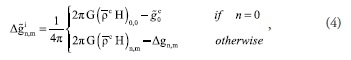
where Y_n,m is the (fully-normalised) surface spherical harmonic function of degree n and order m . The density distribution function p'^c equals p'^c=p^con land and ocean density contrast is defined as:p'^c=p^c-p^w ; where p^c is wareference crust density and p^w mean saltwater density. Ice and sediment density contrasts were defined relative to reference crust density p^c . Nominal (zero-degree) compensation attraction g≈₀^c stipulated at the sphere of radius R was computed as from (Sjöberg, 2009):

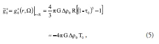
where t₀=T₀,R and T₀ and Δp₀ are the adopted nominal mean values of Moho depth and density contrast, respectively.

Estimation principle 

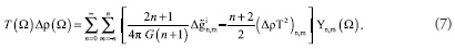
Least-squares analysis was used for estimating T and Δp . The linearised observation equation involved expanding the integral term on the left-hand side of equation (1) into a Taylor series. The subsequent substitution of the first two terms in the series for sⁿ⁺³ from equation (3) to equation (1) yielded (Sjöberg and Bagherbandi, 2011):

From equation (5), the linearised observation equation for product T Δρ was found in the following form:

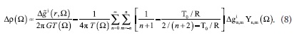
Approximation of term (ΔpT²⁾ in equation (7) by (ΔpT)_nm yielded the linearised observation equation for Δρ in the following form:

Least-squares analysis combined the estimated product of T and Δp with a priori values t and k of such parameters for obtaining improved estimates of T and Δp. The system of observation equations was given in the following vector-matrix form:

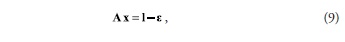
where ε is the vector of residuals. Parameter vector x and observation vector l read:

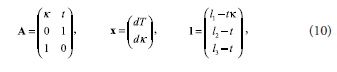
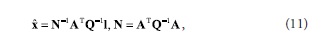
Elements l₁, l₂ and l₃ of the observation vector l were formed, respectively, by observables TΔp, Δp and T. Parameter vector x was defined for unknown corrections and dT to a priori (initial) values of T and Δp. The solution of normal equations was found by solving:

Covariance matrix Q_x of the estimated parameters was computed from:

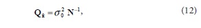
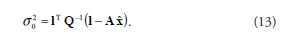
where unit weight variance σ²₀ reads was:

Data acquisition

The computation of isostatic gravity anomalies over the study area of Antarctica required the application of gravity corrections due to rough topography, continental ice sheet and variable geological structure (mainly large sediment deposits). The three largest mountain ranges on the Antarctic continent are the Transantarctic Mountains, the West and East Antarctica ranges. The Transantarctic Mountains is formed by a mountain range extending, with some interruptions, across the continent from Cape Adare in northern Victoria Land to Coats Land. These mountains serve as the natural geographical division between East and West Antarctica. Absolute maxima of topographic gravity correction in this part of the world reach ≈400 mGal (Tenzer et al., 2009). Approximately 98% of the land in Antarctica is covered by the continental ice sheet, thickness exceeding 2 km, while only about 0.32% of the land is ice-free. Maximum ice thickness is 4,776 m. The ice mass thus represents a significant contribution to the gravity field. Another significant gravity field contribution along the continental shelf of Antarctica is due to the presence of large sedimentary basins. Additional large sedimentary deposits exist inland of Antarctica (see Studinger et al., 2003; Bamber et al., 2006). Tenzer et al., (2010, 2012) have demonstrated that ice and sediment stripping corrections to gravity data in Antarctica reach about 300 mGal and 60 mGal, respectively.

The global geopotential model (GOCO02S), the global topographic/bathymetric model (DTM2006.0), ice-thickness data for Antarctica (assembled by the BEDMAP project; Lythe et al., 2001) and sediment density and thickness data from the global crustal model (CRUST2.0) were used in this study to compute isostatic gravity anomalies over the study area of Antarctica bounded by parallel 60 arc-deg of southern geographical latitude. All gravity computations were realized on a 2×2 arc-deg surface grid. Coefficients from the combined GRACE and GOCE satellite global geopotential model GOCO02S (Goiginger et al., 2011) with a spectral resolution complete to degree 180 spherical harmonics were used for producing gravity anomalies. Refined Bouguer gravity anomalies were obtained after applying Bouguer gravity reductions to GOCO02S gravity anomalies. The spherical Bouguer gravity reduction was computed using coefficients from the global topographic/bathymetric model DTM2006.0 (Pavlis et al., 2007) complete to spherical harmonic degree 180. The average density of upper continental crust 2,670 kg/m³ (Hinze, 2003) was adopted as reference crust density. The ocean density contrast 1,643 kg/m³ corresponds to mean seawater density 1,027 kg/m³, Updated 5×5 arc-min ice-thickness data for Antarctica assembled by the BEDMAP project were used to compute the ice (density contrast) stripping gravity correction. The ice stripping gravity correction was computed with a spectral resolution complete to degree/order 180. The ice density contrast 1,753 kg/m³ corresponds to glacial ice density 2,670 kg/m³ (Cutnell and Kenneth, 1995). CRUST2.0 sediment thickness and density data (on 2×2 arc-deg grid) were used for computing the sediment (density contrast) stripping gravity correction with a spectral resolution complete to degree/order 90. CRUST2.0 (Bassin et al., 2000) was compiled and administered by the US Geological Survey and the Institute for Geophysics and Planetary Physics at the University of California. CRUST2.0 is an upgrade of CRUST5.1 (Mooney et al., 1998).

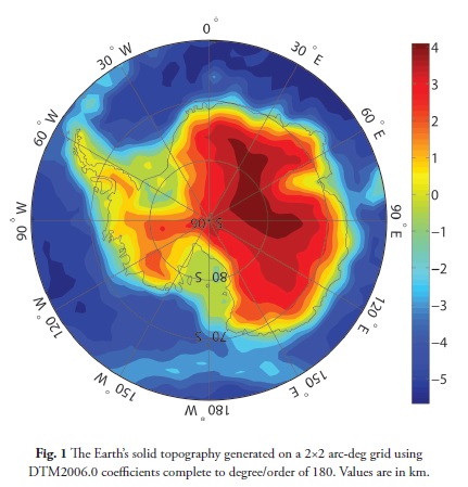
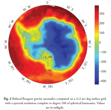
The Earth's solid topography (i.e. topographical heights onshore and bathymetric depths offshore) generated on a 2×2 arc-deg grid using the DTM2006.0 coefficients complete to degree/order of 180 is shown in Figure 1. Maximum topographical heights over the study area reach 4.1 km and maximum bathymetric depths are 5.7 km. Regional map of refined Bouguer gravity anomalies is shown in Figure 2, values were between -457 and 419 mGal (mean = -43 mGal; standard deviation = 286 mGal). Gravity maxima were found over areas of deepest oceans, and toand gravity minima were located throughout the central part of East Antarctica.

Results

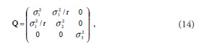
The combined least-squares method was used for a simultaneous estimation of Moho depth and density contrast. The solution was obtained by solving the system of normal equations, which was defined in equation (11). The observation vector l in equation (10) was formed by three observation types l₁=TΔp (eqn. 7), l₂₌Δp (eqn. 8), and l₃=T_s The initial values of Moho depths T_s were taken from CRUST2.0 The variance-covariance matrix Q in the least-squares estimation model (in eqn. 11) was computed from (cf. Sjöberg and Bagherabndi, 2011):

where σ₁ and σ₃ are the standard errors of TΔp and T, respectively, and σ₂² =σ₁² /t² +σ₃²(TΔp)²/t⁴

The standard error σ1 of Δp was computed using the following expression:

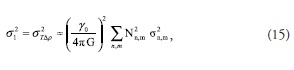
where y₀ is normal gravity,N_nm=(2n+1)(n-1)/(n+1) , and σ_nm²error degree potential coefficients. Since CRUST2.0 Moho depths were not provided with a standard error model, relative uncertainties (i.e. standard errors σ₃) of CRUST2.0 Moho depths of 20% were assumed in forming the matrix Q.

Estimated Moho density contrast taken relative to 2,670 kg/m³ crust density are shown in Figure 3. The density contrast, was found to be between 160 and 682 kg/m³ (mean = 477 kg/m³, standard deviation = 128 kg/m³).

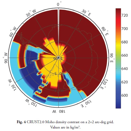
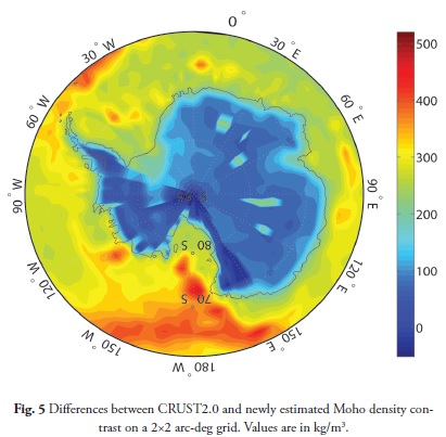
Estimated Moho density contrast was compared with CRUST2.0. CRUST2.0 Moho density contrast was computed from CRUST2.0 upper mantle densities relative to 2,670 kg/m³ crust density. CRUST2.0 Moho density contrast is shown in Figure 4. Differences between both Moho density contrasts are shown in Figures 5. Whereas large variations of Moho density contrast were estimated using the combined least-squares approach (Fig. 2), the range of CRUST2.0 values was within 580 and 730 kg/m³ (Fig. 4). Such large discrepancies (shown in Fig. 5) were likely caused by a low quality of CRUST2.0 upper mantle density, especially under oceanic crust. CRUST2.0 upper mantle density under oceanic crust was significantly overestimated. CRUST2.0 Moho density contrast under the Antarctic continental crust had a good agreement with our estimates, differences mostly being within ±100 kg/m³.

Discussion

Moho density contrast differs significantly in East and West Antarctica (see Fig. 3). Moho density contrast maxima are situated throughout the central part of East Antarctica with the extension under the Transantarctic mountain range. Moho density contrast there exceeded 500 kg/m³. Moho density contrast beneath West Antarctica was less pronounced. A typical range was between 400 and 500 kg/m³, except for local maxima in the central part of Antarctic Peninsula, where values reached ≈550 kg/m³.

Ritzwoller et al., (2001) and Block et al., (2009) have estimated that average crust thickness in the West Antarctica was ≈27 km. Average crust thickness of ≈40 km was estimated for East Antarctica, with maximum crust thickness being ≈45 km. These large differences could be explained by different tectonic and geological compositions of West and East Antarctica. Dalziel and Elliot (1982) proposed that East Antarctica is a single tectonic block formed predominantly by Craton. Several smaller crust fragments forming West Antarctica have been moved and further reconfigured with respect to East Antarctica and each other. Ritzwoller et al., (2001) and Morelli and Danesi (2004) have analysed shear wave velocities over the whole of Antarctica. They found significant differences in mantle structure characterised by a low velocity in the West Antarctica while a high velocity was detected in the mantle of East Antarctica, with a transition occurring below the Transantarctic Mountains. Unlike most of similar mountain ranges, this mountain range was formed in the absence of collision tectonic forces (ten Brink et al., 1997). Several theories have been proposed explaining possible mechanisms for their formation. Models have included thermal buoyancy from an underlying positive temperature anomaly in upper mantle (ten Brink et al., 1997), thicker crust giving the origin to an isostatically buoyant load (Studinger et al., 2004) or possible collapse of a high-standing plateau with subsequent uplift and denudation (Bialas et al., 2007). The latest models based on integrated geophysical analysis assume that multiple mechanisms have contributed to the uplift of the Transantarctic Mountains (cf. Studinger et al., 2004; Lawrence et al., 2006).

Despite the central part of East Antarctica being characterised by large variation in continental ice- sheet thickness and rough bedrock topography of basins and mountain ranges including sub-glacial mountains, significant variations in Moho density contrast were almost absent (see Fig. 3). Prevailing homogenous Moho density contrast there could be explained by a more uniform geological structure than that of West Antarctica. The location of the largest local density contrast anomalies correspond to the Gamburtsev subglacial mountains, Aurora Basin and Dronning Maud Land. Block et al., (2009) have reported decreasing crust thickness on the margins of East Antarctica due to rifting events that separated Antarctica from the other Gondwana landmasses, with the most pronounced signature occurring on the coast of Dronning Maud Land. This trend was not clearly seen in spatial pattern of Moho density contrast; instead, large Moho density contrast variations across the East Antarctic continental margin could be explained by significantly different geological composition between continental and oceanic crusts, involving typically thick and less dense continental crust compared to thin and heavier oceanic crust.

Distinctive features in the map of Moho density contrast geographically correspond to the West Antarctic Rift in West Antarctica;Moho density contrast there being typically 400 to 450 kg/m³. Similar density contrast was found beneath the Ross Embayment. A possible explanation for these small values in Moho density contrast could be provided by geological structure dominated by volcanic activity occurring since (at least) the early Cenozoic. Holocene volcanism continues in the Ross Embayment (Kiele et al., 1983; Blankenship et al., 1993; Behrendt et al., 1994). According to Behrendt et al., (1994) the main rifting phase occurred between 105 and 85 Ma but episodic extension continued into the Cenozoic. Extension within the rift system has left most of West Antarctica below sea level, with the exception of Marie Byrd Land and parts of the Antarctic Peninsula. It is assumed that this represents remains of a continuously propagating rift that started during the Jurassic period when Africa separated from East Antarctica and proceeded clockwise to its present location in the Ross Embayment and West Antarctica. The almost complete absence of recent seismic activity suggests that there might not be any undergoing active extension of the rift zone (Cande et al., 2000). Local maxima of the Moho density contrast exceeding ≈500 kg/m³ in West Antarctica were found beneath Marie Byrd Land. The lithospheric structure there is characterised by topographic doming due to localised hot spot activity (Hole and LeMasurier, 1994; Winberry and Anandakrishnan, 2004). Moho density contrast was typically less than ≈350 kg/m³ beneath oceanic crust; minima were found along the Pacific Antarctic mid-oceanic ridge. Moho density contrast there was estimated to be as low as 160 kg/m³, corresponding to 2,830 kg/m³ density for the youngest oceanic lithosphere (Müller et al., 2008). Similar density values have also been found between Antarctic and South-American continental tectonic plates, which were separated by a newly-formed oceanic lithosphere.

Conclusions

Spatial variations of Moho density contrast resembled major features of the Antarctic tectonic plate configuration and its geological composition. Density contrast maxima were found throughout the central part of East Antarctica with the extension under the Transantarctic mountain range. Moho density contrast there often exceeded ≈500 kg/m³, maxima being 682 kg/m³. Density contrast maxima were found under mountainous ranges and areas covered by the largest continental ice sheet. These locations are also characterised by the largest thickness of the Antarctic continental crust, Moho depths there reached ≈40 km. According to our estimation, Moho density contrast beneath West Antarctica was typically 400 to 500 kg/m³, except for local maxima (≈550 kg/m³) in the central part of Antarctic Peninsula. Local minima (400-450 kg/m³) beneath the West Antarctic Rift and the Ross Embayment are likely attributed to volcanic compositions throughout this divergent tectonic zone. The largest variations of Moho density contrast were found across the East Antarctic continental margin. Moho density contrast beneath the oceanic crust was typically less than ≈350 kg/m³. The extreme minima were detected along the Pacific Antarctic mid-oceanic ridge.

References

Adams, R.D. (1971). Reflections from discontinuities beneath Antarctica. Bulletin of the Seismological Society of America 61, 5, 1441-1451.         [ Links ]

Bamber, J. L., Ferraccioli, F., Joughin, I., Shepherd, T., Rippin, D. M., Sigert, M. J. and Vaughan, D. G. (2006) East Antarctic ice stream tributary underlain by major sedimentary basin. Geology 34, 1, 33-36.         [ Links ]

Bannister, S., Yu, J., Leitner, B. and Kennett, B. L. N. (2003). Variations in crustal structure across the transition from West to East Antarctica Southern Victoria Land. Geophys. J. Int. 155, 870-884.         [ Links ]

Bassin, C., Laske, G. and Masters, T. G. (2000). The current limits of resolution for surface wave tomography in North America. EOS Trans AGU 81: F897.         [ Links ]

Behrendt, J. C., LeMasurier, W. E., Cooper, A. K., Tessensohn, F., Trehu, A., and Damaske, D. (1991). Geophysical studies of the West Antarctic Rift System. Tectonics 10, 1257-1273.         [ Links ]

Bentley, C. R. and Ostenso, N. A. (1962). On the paper of F.F. Evison, C.E. Ingram, R.H. Orr, and J. H. LeFort, (1962), Thickness of the Earth's crust in Antarctica and surrounding oceans. Geophys J. R. Astron. Soc. 6, 292-298.         [ Links ]

Bialas, R. W., Buck, W. R., Studinger, M. and Fitzgerald, P. (2007). Plateau collapse model for the Transantarctic Mountains West Antarctic Rift System: Insights from numerical experiments. Geology 35, 8, 687-690.         [ Links ]

Blankenship, D., Bell, R. E., Hodge, S. M., Brozena, J. M., Behrendt, J. C. and Finn, C. A. (1993). Active volcanism beneath the West Antarctic ice sheet and implications for ice-sheet stability. Nature 361, 526-528.         [ Links ]

Block, A. E., Bell, R. E. and Studinger, M. (2009). Antarctic crustal thickness from satellite gravity: Implications for the Transantarctic and Gamburtsev Subglacial Mountains. Earth and Planetary Science Letters 288, 1-2, 194-203.         [ Links ]

Cande, S. C., Stock, J. M., Müller, R. D. and Ishihara, T. (2000). Cenozoic motion between East and West Antarctica. Nature 404, 145-150.         [ Links ]

Cutnell, J. D. and Kenneth, W. J. (1995). Physics, 3rd Edition, Wiley, New York.         [ Links ]

Dalziel, I. W. D. and Elliot, D. H. (1982). West Antarctica; problem child of Gondwanaland. Tectonics 1, 1, 3-19.         [ Links ]

Dewart, G. M. and Toksoz, M. N. (1965). Crustal structure in East Antarctica from surface wave dispersion. Geophys. J., R. Astron. Soc. 10, 127-139.         [ Links ]

Evison, F. F., Ingham, C. E., Orr, R. H. and Le Fort, J. H. (1960). Thickness of the earth's crust in Antarctica and the surrounding oceans. Geophys. J. 3, 289-306.         [ Links ]

Forsyth, S. W., Ehrenbarda, R. L. and Chapin, S. (1987). Anomalous upper mantle beneath the Australian-Antarctic discordance. Earth Planet. Sci. Lett. 84, 471-478.         [ Links ]

Goiginger, H., Rieser, D., Mayer-Guerr, T., Pail, R., Schuh, W.-D., Jäggi, A. and Maier, A. (2001). GOCO, Consortium: The combined satellite-only global gravity field model GOCO02S; European Geosciences Union General Assembly 2011, Wien, 04.04.2011.         [ Links ]

Hinze, W. J. (2003). Bouguer reduction density, why 2.67? Geophysics 68, 5, 1559-1560.         [ Links ]

Hole, M. J. and LeMasurier, W.E. (1994). Tectonic controls on the geochemical composition of Cenozoic alkali basalts from West Antarctica. Contrib. Mineral. Petrol. 117, 187-202.         [ Links ]

Ito, K. and Ikami, A. (1986). Crustal structure of the Mizuho Plateau, East Antarctica, from geophysical data. J. Geodyn. 6, 285-296.         [ Links ]

Kiele, J., Marshall, D. L., Kyle, P. R., Kaminuma, K., Shibuya, K. and Dibble, R. R. (1983). Volcanic activity associated and seismicity of Mount Erebus 1982-1983. Antarct. J. U.S. 18, 41-44.         [ Links ]

Knopoff, L. and Vane, G. (1978). Age of East Antarctica from surface wave dispersion. Pure Appl. Geophys. 117, 806-816.         [ Links ]

Kogan, A. L. (1972). Results of deep seismic soundings of the earth's crust in East Antarctica, in: Antarctic Geology and Geophysics, Adie, R.J. (Ed.), pp. 485-489, Universitetsforlag, Oslo.         [ Links ]

Kovach, R. L. and Press, F. (1961). Surface wave dispersion and crustal structure in Antarctica and the surrounding oceans. Ann. Geofis. 14, 211-224.         [ Links ]

Lawrence, J. F., Wiens, D. A., Nyblade, A., Anandakrishnan, S., Shore, P. J. and Voigt, D. (2006). Crust and upper mantle structure of the Transantarctic Mountains and surrounding regions from receiver functions, surface waves, and gravity: implications for uplift models. Geochem. Geophys. Geosyst. 7.         [ Links ]

Llubes, M., Florsch, N., Legresy, B., Lemoine, J. M., Loyer, S., Crossley, D. and Remy, F. (2003). Crustal thickness in Antarctica from CHAMP gravimetry. Earth Planet. Sci. Lett. 212, 103-117.         [ Links ]

Lythe, M. B. and Vaughan, D. G., BEDMAP consortium (2001). BEDMAP; a new ice thickness and subglacial topographic model of Antarctica. J. Geophys. Res., B, Solid Earth Planets 106, 6, 11,335-11,351.         [ Links ]

Morelli, A. and Danesi, S. (2004). Seismological imaging of the Antarctic continental lithosphere: a review. Glob. Planet. Change 42, 155-165.         [ Links ]

Mooney, W. D., Laske, G. and Masters, T. G. (1998). CRUST 5.1: a global crustal model at 5x5 deg. J. Geophys. Res. 103, 727-747.         [ Links ]

Müller, R. D., Sdrolias, M., Gaina, C. and Roest, W. R. (2008). Age, spreading rates and spreading symmetry of the world's ocean crust. Geochem. Geophys. Geosyst. 9, Q04006.         [ Links ]

Okal, E. A., 1981. Intraplate seismicity of Antarctica and tectonic implications. Earth Planet. Sci. Lett., 52, 397-409.         [ Links ]

Pavlis, N. K., Factor, J. K. and Holmes, S. A. (2007). Terrain-Related Gravimetric Quantities Computed for the Next EGM, in: Gravity Field of the Earth, Kiliçoglu A., Forsberg, R. (Eds.), Proceedings of the 1st International Symposium of the International Gravity Field Service (IGFS), Harita Dergisi, Special Issue No. 18, General Command of Mapping, Ankara, Turkey.         [ Links ]

Reading, A. M. (2006). The seismic structure of Precambrian and early Paleozoic terranes in the Lambert Glacier region East Antarctica. Earth Planet. Sci. Lett. 244, 44-57.         [ Links ]

Ritzwoller, M. H., Shapiro, N. M., Levshin, A. L. and Leahy, G. M. (2001). Crustal and upper mantle structure beneath Antarctica and surrounding oceans. J. Geophys. Res., B, Solid Earth Planets 106, 12, 30,645-30,670.         [ Links ]

Rouland, D., Xu, S.H. and Schindele, F. (1985). Upper mantle structure in the southeast Indian Ocean: A surface wave investigation. Tectonophysics, 114, 281-292.         [ Links ]

Roult, G., Rouland, D. and Montagner, J. P. (1994). Antarctica II: Upper mantle structure from velocities and anisotropy. Phys. Earth Planet. Inter. 84, 33-57.         [ Links ]

Sjöberg, L. E. (2009). Solving Vening Meinesz-Moritz Inverse Problem in Isostasy. Geophys. J. Int. 179, 3, 1527-1536.         [ Links ]

Sjöberg, L. E., Bagherbandi, M. (2011). A Method of Estimating the Moho Density Contrast with A Tentative Application by EGM08 and CRUST2.0. Acta Geophysica 58, 1-24.         [ Links ]

Studinger, M., Karner, G. D., Bell, R. E., Levin, V., Raymond, C. A. and Tikku, A. A. (2003). Geophysical models for the tectonic framework of the Lake Vostok region East Antarctica. Earth Planet. Sci. Lett. 216, 4, 663-677.         [ Links ]

Studinger, M., Bell, R. E., Buck, W. R., Karner, G. D. and Blankenship, D. (2004). Sub-ice geology inland of the Transantarctic Mountains in light of new aerogeophysical data. Earth Planet. Sci. Lett. 220, 3-4, 391-408.         [ Links ]

Studinger, M., Bell, R. E., Fitzgerald, P. and Buck, W. R. (2006). Crustal architecture of the Transantarctic Mountains between the Scott and Reedy Glacier region and South Pole from aero-geophysical data. Earth Planet. Sci. Lett. 250, 1-2, 182-199.         [ Links ]

Ten Brink, U. S., Hackney, R. I., Bannister, S., Stern, T. and Makovsky, Y. (1997). Uplift of the Transantarctic Mountains and the bedrock beneath the East Antarctic ice sheet. J. Geophys. Res., Solid Earth 102, B12, 27,603-27,621.         [ Links ]

Tenzer, R., Hamayun and Vajda, P. (2009). Global maps of the CRUST2.0 crustal components stripped gravity disturbances. J. Geophys. Res. 114, B, 05408.         [ Links ]

Tenzer, R., Abdalla, A., Vajda, P. and Hamayun (2010). The spherical harmonic representation of the gravitational field quantities generated by the ice density contrast. Contributions to Geophysics and Geodesy 40, 3, 207-223.         [ Links ]

Tenzer, R., Novák, P., Hamayun and Vajda, P. (2012). Spectral expressions for modelling the gravitational field of the Earth's crust density structure. Studia Geophys. Geodaet.; doi: 10.1007/s11200-011-0023-7        [ Links ]

Vening Meinesz, F. A. (1931). Une nouvelle méthode pour la réduction isostatique régionale de l'intensité de la pesanteur. Bull. Geod. 29, 33-51.         [ Links ]

Winberry, J. P. and Anandakrishnan, S. (2004). Crustal structure of the West Antarctic Rift System and Marie Byrd Land Hotspot. Geology, 32, 11, 977-980.         [ Links ]