SEISMOLOGY

A methodology for the analysis of the Rayleigh-wave ellipticity

V. Corchete

Higher Polytechnic School, University of Almeria, 04120 ALMERIA, Spain

Manuscript received: 23/10/2012
Accepted for publication: 06/08/2013

ABSTRACT

In this paper, a comprehensive explanation of the analysis (filtering and inversion) of the Rayleigh-wave ellipticity is performed, and the use of this analysis to determine the local crustal structure beneath the recording station is described. This inversion problem and the necessary assumptions to solve are described in this paper, along with the methodology used to invert the Rayleigh-wave ellipticity. The results presented in this paper demostrate that the analysis (filtering and inversion) of the Rayleigh-wave ellipticity is a powerful tool, for studying the local structure of the crust beneath the recording station. Therefore, this type of analysis is very useful for studies of seismic risk and/or seismic design, because it provides local earth models in the range of crustal depths.

Key words: Ellipticity, multiple filter technique (MFT), time variable filtering (TVF), inversion.

RESUMEN

En este artículo, será realizada una explicación fácil de comprender del análisis (filtrado e inversión) de la elipticidad de la onda Rayleigh, así como, de su aplicación para determinar la estructura local bajo la estación de registro. Este problema de inversión y los necesarios supuestos para resolverlo, serán descritos en el artículo, juntamente con la metodología utilizada para invertir la elipticidad de la onda Rayleigh. Los resultados presentados en este artículo mostrarán que el análisis (filtrado e inversión) de la elipticidad de la onda Rayleigh es una poderosa herramienta, para estudiar la estructura local de la corteza terrestre bajo la estación de registro, siendo este tipo de análisis muy útil para estudios de riesgo y/o diseño sísmico, porque proporciona modelos de Tierra locales en el rango de profundidades corticales.

Palabras clave: Elipticidad; filtro técnico múltiple; filtrado temporal variable; inversión.

1. Introduction

As it is well known, many surface-wave studies have been devoted to obtaining the structure of the earth (crust and upper mantle) from the surface-wave dispersion analysis (filtering and inversion). The surface-wave dispersion varies along the propagation path, in a manner related to the earth structure that is crossed by these waves. Therefore, the surface-wave dispersion analysis is a good tool for studying the most important features of the earth structure. In particular, in the Iberian region, several shear-velocity models (earth models) of the crust and upper mantle have been obtained by Corchete et al. (1993, 1995), from the analysis of Rayleigh-wave dispersion. This analysis consisted of filtering and inverting the Rayleigh-wave dispersion, to obtain the variation in the shear-wave velocity versus depth. Nevertheless, the Rayleigh-wave dispersion is dependent upon the propagation path of these waves, and it does not depend (primarily) upon the local crustal structure beneath the recording station (seismic station). As a consequence of this, the Rayleigh-wave dispersion analysis could not be used to determine earth models (crustal models) beneath local areas (small areas), such as the area in the vicinity of the seismic station (Malischewsky et al., 2010; Tuan et al., 2011).

At this point, the analysis (filtering and inversion) of the Rayleigh-wave ellipticity gain importance, because Sexton et al. (1977) have shown that the Rayleigh-wave ellipticity depends primarily upon the local crust structure and that it does not exhibit azimuthal dependence, for a period range of 10 to 50 s. Thus, for this period range, the observed ellipticity is primarily controlled by the local crustal geology beneath the seismic station, it does not depend upon the propagation path of the Rayleigh waves. This basic property of the ellipticity means that the ellipticity analysis is a very useful tool for obtaining local crustal models, which can be used to determine the site and/or local effects in studies of seismic risk and/or seismic design (Lee et al., 2003; Rastogi et al., 2011).

For this reason, it is very desirable to develop a methodology for the analysis of the Rayleigh-wave ellipticity that can be used to determine the local crustal structure beneath the recording station (seismic station). This analysis consists of filtering and inverting Rayleigh-wave ellipticity curves to obtain S-velocity models (variations in shear-wave velocity versus depth). Thus, the goal of this paper is to provide a comprehensive explanation of the analysis (filtering and inversion) of the Rayleigh-wave ellipticity, devoting particular attention to the inversion problem and the assumptions necessary to solve it.

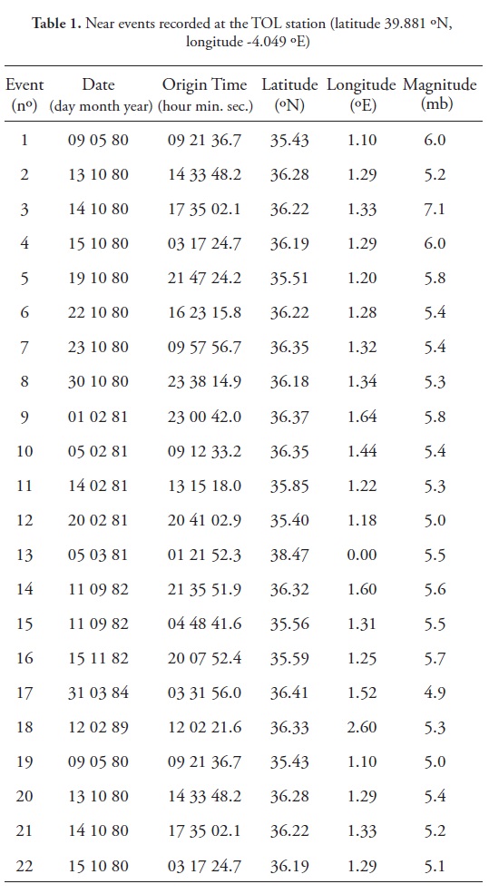
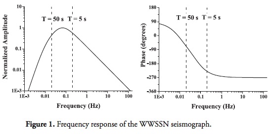
2. Data

In this type of study, the primary data used are seismograms. The seismograms used in this study correspond to 22 earthquakes (Table 1) that occurred in the neighboring region of the Iberian Peninsula. These earthquakes were registered by the WWSSN station TOL located in Iberia (latitude 39.881 ^ºN, longitude -4.049 ^ºE). The records of this station are considered to be suitable for this study, because the period range of best registration for the WWSSN seismograph is between 5 and 50 s (the period range in which the amplitude spectrum is maximized), as seen in Figure 1 (Kulhánek, 1990). This period range (from 5 to 50 s) is most suitable for exploring the elastic structure of the earth for a depth range from 0 to 50 km, which coincides with the goal of this study. Only earthquake traces in which there exist well-developed Rayleigh wave trains with a very clear dispersion are considered to ensure the reliability of the results. Logically, instrumental correction must be taken into account to eliminate the time lag introduced by the seismograph system and all distortions produced by the instrument (Bath, 1982; Kulhánek, 1990). This correction recovers the true amplitude and phase of the ground motion, allowing the analysis of the true ground motion attributable to the Rayleigh wave. For this reason, all traces considered in this study have been corrected for the instrument response.

3. Computation of the observed ellipticity

It is known that the observed ellipticity of a Rayleigh wave can be calculated using the formula (Aki and Richards, 1980; Ben-Menahem and Singh, 1981)

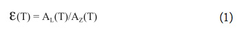
where A_L(T) and A_Z(T) are the instrument-corrected spectral amplitudes of the longitudinal (also called radial) and vertical seismograms for the period T (Sexton et al., 1977). Nevertheless, the use of equation (1) poses some practical difficulties. The first difficulty of formula (1) is that the ellipticity values can be calculated only for the periods generated by the Fast Fourier Transform (FFT). Thus, many values can be computed for short periods, but only a few values can be computed for long periods. The second important difficulty of formula (1) is the presence of spectral holes in A_Z(T), the spectral amplitude of the vertical seismogram. A spectral hole is a small value (near zero) that can exist, for some period T, in the spectral amplitude. This small value, when introduced into the denominator of a spectral ratio such as the ratio given by formula (1), produces a very large value (near infinite) for this ratio (ε(T) → ∞ for some period T in which A_Z(T) → 0). In a spectral hole, the formula (1) has no physical meaning and it cannot be applied. Spectral holes can be produced by noise or other such undesirable perturbations that typically are present in all seismograms.

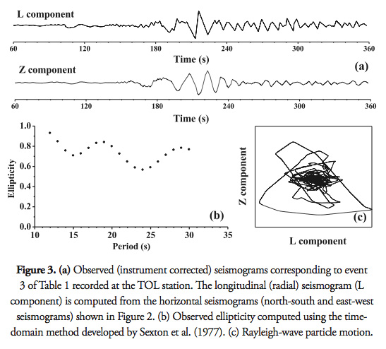
Because of the above-mentioned difficulties, the use of equation (1) directly is not suitable for a systematic computation; instead, a time-domain method, based on the Multiple Filter Technique (MFT) of Dziewonski et al. (1969), is more suitable for the systematic computation of the observed ellipticity. Thus, the time-domain method developed by Sexton et al. (1977) is used here for the computation of the observed ellipticity, instead of the spectral ratio given by formula (1). Figure 2 shows the seismograms recorded at the TOL station for event 3 (listed in Table 1). These records are used to illustrate the time-domain method applied in this study for the computation of the observed ellipticity. Figure 3 shows the results obtained by applying the method developed by Sexton et al. (1977), to the seismograms shown in Figure 2. It should be noted that noise and other undesirable perturbations, which are always present in the data (Figure 3c), can introduce errors into the computation of the observed ellipticity.

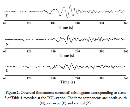
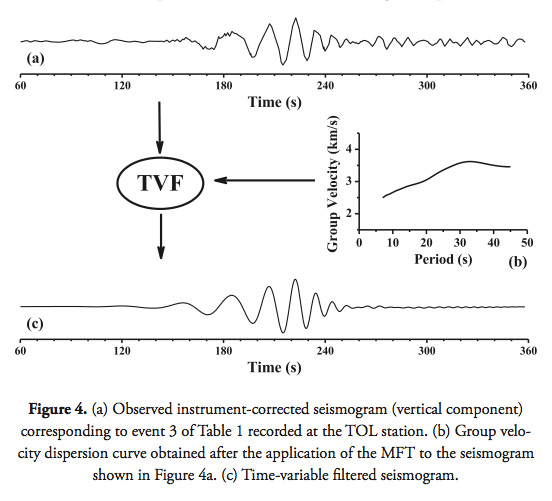
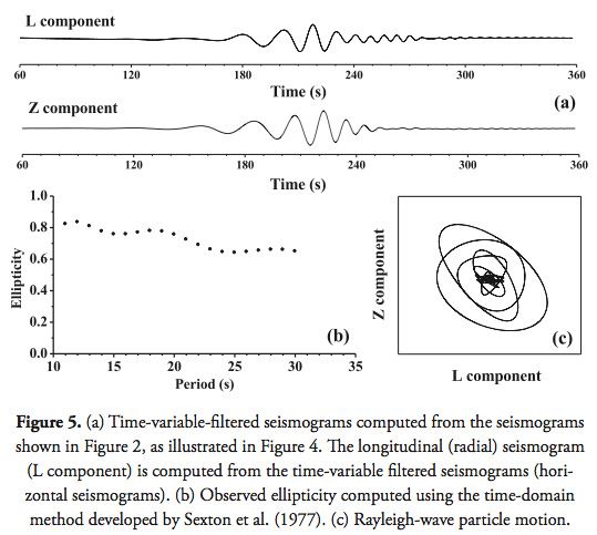
The majority of this noise and undesirable perturbations can be removed from the data (seismograms) using the Time Variable Filtering (TVF) technique. TVF is a filtering technique that produces a smooth seismogram (a time-variable-filtered seismogram), in which all effects of noise, higher modes and other undesirable perturbations have been removed (Cara, 1973). This technique can be used in combination with the MFT, as described by Corchete et al. (2007), to obtain better results than those obtained using the MFT only. The use of TVF in this study is illustrated in Figure 4, in which the vertical seismogram shown in Figure 2 has been time-variable filtered. This technique was applied to all seismograms used in this study to compute the observed ellipticity, as shown in Figure 5. A comparison between Figures 3 and 5 illustrates the improvement achieved by the combination of the MFT and TVF (Figure 5) versus the application of the MFT only (Figure 3). The particle motion (ground motion) attributable to the Rayleigh wave is much clearer in Figure 5c than in Figure 3c, which confirms that the observed ellipticity presented in Figure 5b is more reliable than the one presented in Figure 3b.

Once the ellipticity curve (observed ellipticity) for the seismograms of each event listed in Table 1 has been calculated using the above-described combination of filtering techniques (MFT and TVF), an average ellipticity curve (Figure 8c) can be obtained by computing the median of the 22 ellipticity curves calculated for the 22 events listed in Table 1. An estimation of the error on this average ellipticity curve is obtained by computing the standard deviations (1-s error) of the values involved in the calculation of this median.

4. Inversion of the observed ellipticity

Theoretical problem. Once the Rayleigh-wave ellipticity (observed ellipticity) has been obtained, as described in the section above, a relation between the ellipticity and the earth model (given by its characteristic parameters d: layer thickness, α: P-wave velocity, β: S-wave velocity and ρ: density) must be established. Fortunately, this relation exists (and is well known) through the Rayleigh-wave amplitudes in the form (Ben-Menahem and Singh, 1981)

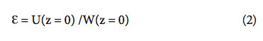
where U(z) and W(z) are the horizontal (also called radial or longitudinal) and vertical amplitudes, respectively. These amplitudes are calculated from an earth model as functions of the depth z, for a given period T, using the forward modelling method described by Abo-Zena (1979) and Aki and Richards (1980). Thus, the theoretical ellipticity (known as the surface ellipticity) defined at z = 0 by formula (2) can be related to an earth model through the general relation

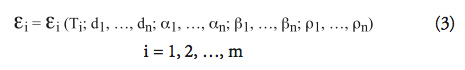
where i is the ith value of the period T (in which the observed ellipticity is calculated), m is the number of values for the period T and n is the number of layers for the earth model under consideration. This layered model is defined by the following parameters: d_j (layer thickness), α_j (P-wave velocity), β_j (S-wave velocity) and ρ_j (density), where the subscript j corresponds to the jth layer of this model.

Linearization of the problem. Equation (3) is a set of m no-linear equations with 4*n unknowns that express the existing relation between the ellipticity and the earth model. Nevertheless, the inverse relation of equations (3) is needed to obtain the values of the model parameters (d_j, α_j, β_j and ρ_j for j varying from 1 to n) from the observed data (ε_i for i varying from 1 to m). This inverse relation can be very difficult to obtain from equations (3) in absence of any simplification. The simplification approach used in this study is the method developed by Dorman and Ewing (1962). This method allows the linearization of equations (3) using the partial derivatives of the ellipticity. These partial derivatives are introduced into the problem through the definition of the ellipticity differential, given by

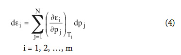
where N (= 4*n) is the total numbers of model parameters and pj is a model parameter (with value d₁,…,d_n; α₁,…,α_n; β₁,…,β_n; ρ₁,…,ρ_n). Then, if an initial model is prepared to produce a theoretical ellipticity curve that is as close as possible to the observed curve, the difference between the theoretical and observed ellipticities can be written as

where ε⁰_i is the observed ellipticity obtained for the ith value of the period T, ε^T_i is the theoretical ellipticity calculated using formula (3) and dei is computed using formula (4). It should be noted that equations (4) and (5) provide an approximate linear relation between the ellipticity and the earth model, when only small perturbations (Δp_j) of model parameters are considered. In this case, a linear relation between the values of the model parameters (d_j, α_j, β_j and ρ_j for j varying from 1 to n) and the observed data (eI for i varying from 1 to m) can be written in the form

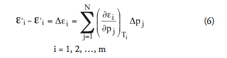
Equations (6) is a set of linear equations that can be inverted to obtain the values of the model parameters from the observed data. Nevertheless, when the total number of parameters N that are taken into consideration is very large, a precise solution for the inverse problem can be very difficult to obtain. For this reason, the total number of parameters must be reduced to the minimum necessary parameters. The total number of parameters can be reduced when only the S-wave velocities are considered in formula (6), i. e. Δp_j = Δβ_j and N = n. Thus, the perturbations (Δp_j) for the P-wave velocity and density are not considered in formula (6) because surface waves are not very sensitive to them (Dorman and Ewing, 1962). Under this final assumption, equation (6) can be inverted if the partial derivatives are evaluated numerically. This numerical evaluation of the partial derivatives can be performed using the approximate relation given by

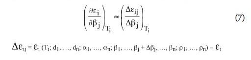
where ε_i is calculated using formula (3) and Δβ_j is a small perturbation (Δβ_j << β_j).

Inversion scheme. Once the forward problem has been linearized using (6) and (7), the inversion of (6) or, equivalently, the inversion of the matrix relation

must be performed, where y = ε⁰ - ε^T, A is given by (7) and x = Δβ. The inverse of the matrix A in relation (8) can be calculated using (Dimri, 1992)

where α is the damping parameter or damping factor and I is the identity matrix. The addition of this factor to the main diagonal of matrix A^TA increases the magnitude of its eigenvalues, thereby avoiding the problems caused by small or zero eigenvalues, which can cause the matrix A^TA to be singular or nearly singular. When the relation called the singular value decomposition (SVD) of A

where the matrices U_p, Λ_p and V_p are described in detail by Aki and Richards (1980) and Dimri (1992). The matrix B defined by formula (10) is called the damped generalized inverse. Then, the linear equations given by (8) can be inverted to obtain x using the expression given in (10) as follows

The product of matrices B and A is called the resolution matrix, and it is obtained as follows

If the resolution matrix given by (12) is the identity matrix, then the solution obtained in this manner is unique and the resolution is perfect. Nevertheless, it should be noted that the addition of the factor α to the main diagonal ensures that the equality BA = I is never reached when the damping factor α is not zero. Therefore, the particular solution that is obtained is never the true solution. The obtained solution is instead a smoothed solution because each model parameter is a weighted mean of the parameters x that define the true model. For this reason, the factor α must be as small as possible to yield the best possible solution, i.e., the particular solution that is as near as possible to the true solution.

The error on the model parameters is given by the corresponding variance (assuming that the data are statistically independent and that the same is true for the model parameters) as follows

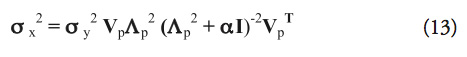
where σ_x² and σ_y² are the variances of the model parameters and the data, respectively.

The inversion scheme proposed in this paper is defined by (10) and it introduces the damping parameter, which degrades the resolution but stabilizes the obtained solution by reducing the variance, as seen in (12) and (13). Thus, an increase in the value of a reduces the error in the determination of the model parameters at the expense of the degradation of the resolution. On the other hand, the inverse given by (10) uses the SVD method instead of the least-squares method, which is used by Dorman and Ewing (1962), because the SVD method provides higher computation accuracy (Keilis-Borok, 1989).

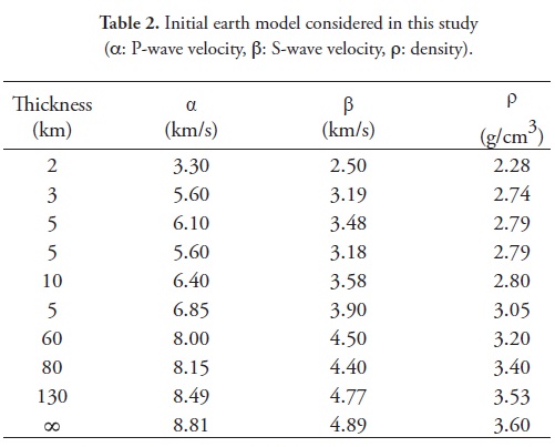
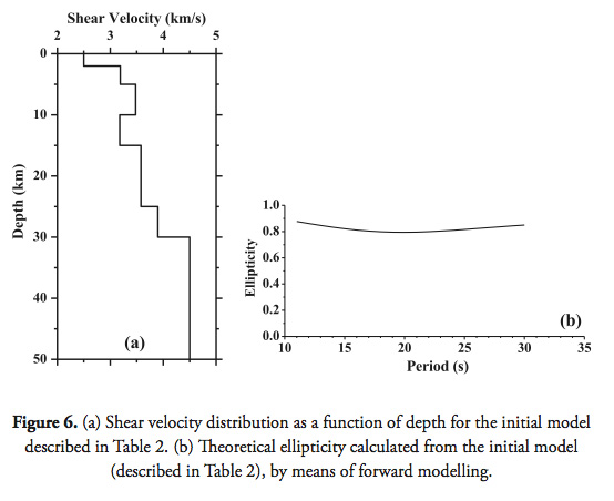
Inversion process. A necessary step that must precede the inversion process is the preparation of an initial model that contains all available information for the study region, including the S-wave, P-wave and density distributions as functions of depth. In this study, this information was obtained from the references provided and is described in section 1. All this information was considered in the preparation of the initial model used to invert the ellipticity curve shown in Figure 8c, which was obtained as described in section 3. The initial model must be prepared to produce a theoretical ellipticity curve that is as close as possible to the observed curve, because the inversion scheme described above considers only small perturbations in the model parameters involved. This method simply conditions the initial model, which is chosen to be as similar as possible to the true earth structure, as represented by all geophysical information available for the study region. The initial model prepared here is described in Table 2, and its shear-wave velocity distribution as a function of depth is plotted in Figure 6a. The calculated theoretical ellipticity is shown in Figure 6b. This curve was obtained using the forward-modelling method described by Abo-Zena (1979) and Aki and Richards (1980).

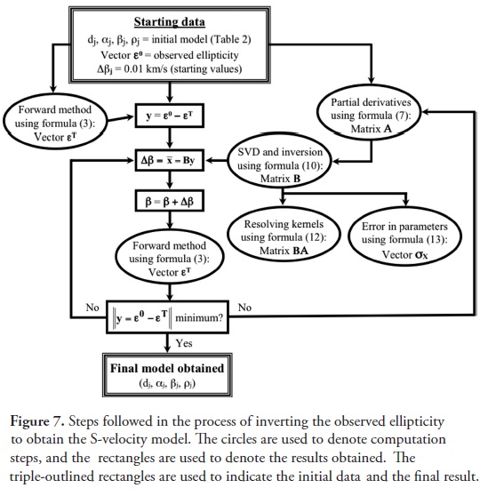
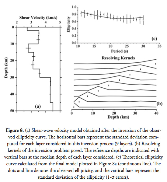
Once the initial model has been prepared, the inversion of the observed ellipticity curve (Figure 8c) can be performed to obtain the corresponding S-velocity model. A computer program based on the above-described inversion scheme, which performs the computation steps shown in the flow chart displayed in Figure 7, was used for this task. The results of this computer program are shown in Figure 8. The S-velocity model shown in Figure 8a is the final obtained model, which was improved iteratively. The iterative improvement in the model is assessed by comparison between the observed ellipticity, considered to be the observed data, and the theoretical ellipticity calculated from the actual model via forward modelling. If each successive curve is closer to the observed ellipticity curve than the previous iteration, the process converges. When the theoretical curve falls within the vertical error bars of the observed data, as seen in Figure 8c, the inversion process is considered to be finished because the obtained shear-velocity model describes the observed curve within its experimental error.

The resolving kernels shown in Figure 8b indicate the reliability of the solution obtained for the considered inverse problem. The resolving kernels are the row vectors of the resolution matrix given by formula (12), and therefore, they are a measure of the exactness of the solution of the inverse problem. Good agreement between the calculated solution and the true solution (which implies the reliability of the estimated solution) is obtained when the absolute maxima of these functions lie at the reference depths. These reference depths are defined as the median depths of each layer considered in the model. The reliability of the solution is also related to the widths of these absolute maxima. The solution identified for the inversion problem is more reliable when the maxima of these resolving kernels are narrower. To achieve this goal and improve the resolution, the number of model layers considered for the inversion must be reduced to be the minimum number of layers that are necessary to obtain a detailed shear-velocity distribution as function of depth, with sufficient precision to describe the observed data within the experimental error (Singh et al., 2011). In this case, the number of layer considered for the inversion (i. e., the total number of model parameters to be perturbed) is n = 9. If a large number of layers are considered, then the number of unknowns is increased but the amount of data remains the same, and the resolution is degraded as a result (Corchete et al., 2007). This effect manifests as resolving kernels with wider absolute maxima and in the lack of coincidence between the maxima of these functions and the reference depths. Another method of improving the resolution is to consider layers with thicknesses that increase with increasing depth, as the resolution worsens. This effect is apparent in Figure 8b: the resolving kernels worsen as the depth increases. The layer thickness considered in our model increases with increasing depth to avoid this effect as much as possible. Thus, the shallow layers are thinner than the deeper layers, which are thicker (Figure 8a).

5. Conclusions

The results presented in this paper demonstrate that the analysis of Rayleigh-wave ellipticity is a powerful tool for investigating the local structure of the crust and upper mantle directly beneath the recording station. This technique can reveal the principal structural features beneath the seismic station because the Rayleigh-wave ellipticity depends primarily upon the local crust structure and does not exhibit azimuthal dependence in the period range of 10 to 50 s. Thus, a general picture of the lithospheric structure beneath the station, in a depth range from 0 to 50 km, can be obtained using this type of analysis. Therefore, the methodology presented in this paper, which consist of filtering and inverting Rayleigh-wave ellipticity curves to obtain S-velocity models (variations in shear-wave velocity versus depth), can be a very useful tool in studies of seismic risk and/or seismic design because it provides local earth models in the range of crustal depths.

Acknowledgements

The author is grateful to Instituto Geográfico Nacional (Madrid, Spain), which provided the seismic data used in this study.

References

Abo-Zena A., 1979. Dispersion function computations for unlimited frequency values. Geophys. J. R. astr. Soc., 58, 91-105.         [ Links ]

Aki K. and Richards P. G., 1980. Quantitative Seismology. Theory and methods. W. H. Freeman and Company, San Francisco.         [ Links ]

Bath M., 1982. Spectral Analysis in Geophysics. Elsevier Science Publishers. Amsterdam.         [ Links ]

Ben-Menahem A. and Singh S. J., 1981. Seismic Waves and Sources. Springer-Verlag. New York.         [ Links ]

Cara M., 1973. Filtering dispersed wavetrains. Geophys. J. R. astr. Soc., 33, 65-80.         [ Links ]

Corchete V., Badal J., Pujades L. and Canas J. A., 1993. Shear velocity structure beneath the Iberian Massif from broadband Rayleigh wave data. Phys. Earth Planet. Inter., 79, 349-365.         [ Links ]

Corchete V., Badal J., Serón F. J. and Soria A., 1995. Tomographic images of the Iberian subcrustal lithosphere and asthenosphere. Journal of Geophysical Research, 100, 24133-24146.         [ Links ]

Corchete V., Chourak M. and Hussein H. M., 2007. Shear wave velocity structure of the Sinai Peninsula from Rayleigh wave analysis. Surveys in Geophysics, 28, 299-324.         [ Links ]

Dimri V., 1992. Deconvolution and inverse theory. Application to geophysical problems. Methods in Geochemistry and Geophysics, 29. Elsevier Science Publishers, Amsterdam.         [ Links ]

Dorman J. and Ewing M., 1962. Numerical inversion of seismic surface wave dispersion data and crust-mantle structure in the New York-Pennsylvania area. Journal of Geophysical Research, 67, 5227-5241.         [ Links ]

Dziewonski A., Bloch S. and Landisman M., 1969. A technique for the analysis of transient seismic signals. Bull. Seism. Soc. Am., 59, 427-444.         [ Links ]

Kulhánek O., 1990. Anatomy of seismograms. Elsevier Science Publishers. Amsterdam.         [ Links ]

Lee W., Kanamori H., Jennings P. and Kisslinger C., 2003. International Handbook of Earthquake and Engineering Seismology. Elsevier, New York.         [ Links ]

Malischewsky P. G., Zaslavsky Y., Gorstein M., Pinsky V., Tran T. T., Scherbaum F. and Flores-Estrella H., 2010. Some new theoretical considerations about the ellipticity of Rayleigh waves in the light of site-effect studies in Israel and Mexico. Geofísica Internacional, 49, 141-152.         [ Links ]

Rastogi B., K., A. P. Singh, B. Sairam, S. K. Jain, F. Kaneko, S. Segawa and J Matsuo, 2011. The Possibility of Site Effects: the Anjar Case, Following the Past Earthquakes in the Gujarat, India. Seismological Research Letters, 82(1): 692-701; DOI 10.1785/gssrl.82.1.692.         [ Links ]

Sexton J. L., Rudman A. J. and Mead J., 1977. Ellipticity of Rayleigh waves recorded in the Midwest. Bull. Seism. Soc. Am., 67, 369-382.         [ Links ]

Singh, A., P., O. P. Mishra, B. K. Rastogi and Dinesh Kumar, 2011. 3-D Seismic Structure of the Kachchh, Gujarat and Its Implications for the Earthquake Hazard Mitigation. Natural Hazards, 57(1): 83-105; DOI 10.1007/s11069-010-9707-2.         [ Links ]

Tuan T. T., Scherbaum F. and Malischewsky P. G., 2011. On the relationship of peaks and troughs of the ellipticity (H/V) of Rayleigh waves and the transmission response of single layer over half-space models. Geophys. J. Int., 184, 793-800.         [ Links ]