GEOTECHNICS

Debris flow susceptibility mapping in a portion of the Andes and Preandes of San Juan, Argentina using frequency ratio and logistic regression models

Esper Angillieri, M.Y.¹

¹CONICET- Gabinete de Neotectónica y Geomorfología, INGEO. Facultad de Ciencias Exactas, Físicas y Naturales,

Universidad Nacional de San Juan. E-mail: yaninaesper@gmail.com

Manuscript received: 22/07/2013
Accepted for publication: 01/11/2013

ABSTRACT

In this study, the frequency ratio and logistic regression models are applied and verified for the analysis of debris flow susceptibility in a portion of the Dry Frontal Andes and Occidental Preandes of San Juan at approximately 30°S latitude, through aninvestigation based on a Geographic Information System (GIS). The site under study covers an area of 2175.9 km² with a debris flow area of 42.45 km². For this purpose, thematic layers including debris flow inventory, lithology, elevation, slope, aspect, and solar radiation were used. The debris flow inventory map was prepared by interpreting aerial photographs and satellite images and was supported by field surveys. Lithology was extracted from an existing geological map. Slope, aspect and solar radiation were calculated from a Digital Elevation Model created from SRTM (Shuttle Radar Topographic Mission) and topographical maps. The relationship between the variables and the debris flow inventory was calculated using the frequency ratio and logistic regression models. Both models helped to produce debris flow susceptibility maps that classified susceptibility into five categories: very low, low, moderate, high and very high. Subsequently, each debris flow susceptibility map was compared with known debris flow locations and tested. The frequency ratio model (accuracy is 82.71%) was more accurate than the logistic regression model (accuracy is 75.64%) for predictons of the high and very high categories.

Key words: Debris flow susceptibility, GIS, San Juan, Argentina

RESUMEN

En este trabajo se aplican, mediante el uso de Sistemas de Información Geográfica, dos modelos estadísticos en la evaluación de la susceptibilidad del terreno a la ocurrencia de flujos de detritos, la relación de frecuencias (F_r) y la regresión logística. El área de estudio comprende un sector de Cordillera Frontal y de Precordillera Occidental a los 30°S de latitud media. Se crearon mapas de elevación, pendiente, insolación, orientaciones, estratigrafía y un inventario de flujos de detritos. Este último, a partir de la interpretación y análisis digital de fotografías aéreas e imágenes satelitales. La estratigrafía fue obtenida a partir de cartas geologicas preexistentes. Las pendientes, orientaciones e insolación fueron calculadas, a partir de un modelo digital de elevaciones. Los mapas de susceptibilidad generados han sido reclasificados en cinco categorías: muy baja, baja, moderada, alta y muy alta. Finalmente, estos mapas, fueron validados espacialmente y como resultado se observa que el modelo Fr predice mejor (82,71%) que la regresión logística (75,64%) para las clases alta y muy alta.

Palabras clave: Susceptibilidad, Flujos de detritos, SIG, San Juan, Argentina.

Introduction

A debris flow is a flow of sediment and water mixture that acts as a continuous fluid driven by gravity, and it attains large mobility from the enlarged void space saturated with water or slurry (Takahashi, 2007)it is. Debris flows are widely recognized as one of the dominant geomorphic processes in the Central Andesis and are strongly correlated with heavy or prolonged rainstorms, often in association with intense snowmelt. Debris flows cause loss of life and property and damage to natural resources and hamper developmental projects, such as roads and communication lines. Because the study area is lowly populated or, in most locations, uninhabited, these events have hardly been documented and rarely damage property. However, most of the small towns in the Department of Iglesia (Figure 1) are situated downstream of river basins from the Frontal Andes (Malimán, Colangüil, Angualasto) or Occidental Preandes (Buena Esperanza). These villages have suffered flash floods and debris flows during every summer period, which has caused material suffered damage, and several casualties have resulted, as evident by events that occurredfor example, during occurrences in 1913, 1944 and 2007 (Angualasto, Buena Esperanza and Malimán). The elongated morphology of the main watersheds, coupled with their significant height difference (promoting rapid runoff), are the most important variables that control flow generation.

Figure 1.

Several authors have studied landslides in Argentina (Fauqué et al., 2000; Moreiras, 2006; Fernández, 2005; Penna et al., 2008; González Díaz, 2009; González Díaz and Folguera, 2009; Perucca and Esper, 2008, 2009a,b).

Debris flow susceptibility mapping aims to differentiate a land surface in homogeneous areas according to the probability of occurrence in an specific area on the basis of local terrain conditions (Varnes, 1978; Brabb, 1984). The debris flow susceptibility analysis was performed by applying the frequency ratio and logistic regression models.

In this study, debris flow susceptibility assessment in a GIS environment is based on a comparison of a debris flow inventory map and conditioning variables (lithology, elevation, slope, aspect, and solar radiation). The debris flow inventory map was prepared by interpreting aerial photographs and satellite images and was supported by field surveys. Slope, aspect and solar radiation were calculated from a Digital Elevation Model created from SRTM (Shuttle Radar Topographic Mission) and topographical maps.

In various papers, models such as frequency ratio and logistic regression have been used for landslide susceptibility. These include studies by Atkinson and Massari (1998); Süzen and Doyuran (2004); Lee (2005); Ayalew and Yamagishi (2005); Lee and Sambath (2006); Nefeslioglu et al. (2008); Kincal et al. (2009); Nandi and Shakoor (2010); Bai et al. (2010, 2011); Chauhan et al. (2010); Das et al. (2010); Oh and Lee (2010); Ercanoglu and Temiz (2011); and Yalcin et al. (2011).

The aim of this study is to prepare debris flow susceptibility maps using the frequency ratio and logistic regression models for a sector of the Andes and PreAndes of San Juan, Argentina. The resulting maps can provide a basis for urbanism, land use planning and would be utilized by public administration offices and insurance companies.

Regional setting

Study area

The territory of interest covers an area of 2175.9 km² in which debris flows have a spatial distribution of 42.45 km². It is located in the middle west of Argentina in northern San Juan Province, Iglesia Department, between latitudes 29°39′–30°9′S and longitudes 68°47′-69°41′W, on the northeast side of the Central Frontal Andes and north of the Occidental PreAndes, which are characterized by high relief with peaks up to 5000 m a.s.l. (Figure 1).

The hillsides rise from 1587 m a.s.l. to 5639 m a.s.l. with average slope angles of 12°. The slopes are very steep in the upper portion (~45°) and are rocky and poorly vegetated. The lower slopes are comprised of talus and relict debris flow deposits.

Climate

The area is characterized by semi-arid conditions with a dry climate, short summers and severe winters with very low temperatures (−18°C to 0°C) and strong winds, and the rainy season normally lasts from November to March. However, the rainfall regime is irregular, with periods of little precipitation and some with lengthy heavy rains. Above 4000 m a.s.l., the precipitation is mainly snow and hail; precipitation events are irregular. The largest amount of rainfall measured during one day was 52 mm on 26 December 1967 with an intensity of 104 mm/h, and the largest amount of rainfall measured in one month was 62.3 mm in January 1993. The annual precipitation of the town of Rodeo is 44.9 mm, but precipitation varies notably with elevation; the annual precipitation for most of the study area is between 100 and 200 mm (Minetti et al., 1986).

According to observations recorded over 42 years in Rodeo, July is the coldest month, with an average temperature of 7.91°C, and the hottest month is January, with temperatures averaging 23.1°C. From 3300 to 4300 m a.s.l., the temperatures are between −18°C to 10°C. Above 4300 m a.s.l., the average temperature in January is below 0°C, and the formation of permafrost is likely.

Geological setting

The area is dconsists of the Cordillera Frontal Ranges and the Precordillera Occidental geological provinces. The Cordillera Frontal is a mountainous system generally running in the north–south direction with peaks up to 5000 m a.s.l. and is composed of a suite of Upper Paleozoic rocks which unconformably overlie a Middle Proterozoic substratum (Ramos, 1999) and highly deformed Lower Paleozoic sedimentary rocks. The oldest stratigraphic unit in the area is a sedimentary unit mainly composed of Upper Carboniferous–Lower Permian dark green mudstones interbedded with sandstones and conglomerates. This unit is overlain unconformably by a Permian–Lower Triassic mesosilicic and silicic volcanic and igneous complex, including pyroclastic, subvolcanic and intrusive rocks, that consists of a lower andesite to dacite section and an upper rhyolitic section. Both units are intruded by medium-grained Triassic grayish granodiorites, which in turn are intruded by pink-red rhyolitic bodies. The sequence continues with an Eocene-Oligocene unit composed of conglomerates, sandstones, multicolor tuffs, andesites, breccia and ignimbrite that rests unconformably on the Permo-Lower Triassic volcanic complex and is intruded by Miocene intrusive rocks of varied composition (granodioritic, andesitic, dacitic, dioritic, and granitic).

The Precordillera, an older orographic system with lower topographical hierarchy, has a general north–south direction and rises up to 3000 m a.s.l. Lower Ordovician sedimentary rocks are the oldest stratigraphic units, composed of limestones, sandstones and lutites, and are observed in the eastern parts of the study area. Devonian conglomerates composed of sandstones and pelites appear in the area, and Carboniferous marine formations (lutites, wakes and conglomerates) are unconformably overlain in sequence.

Along the Iglesia valley, the lithology is represented by Paleogene, Neogene and Quaternary deposits. The Paleogene–Neogene deposits are represented by sedimentary units composed of alluvial and colluvial deposits as well as Miocene argillites.

The Quaternary deposits are formed by gravels, sands, marls, and clays and are restricted to narrow river channels and valleys. was Data were acquired from geologic sheets published by the Servicio Geológico Minero Argentino (Argentine Mining Geologic Service) on a 1:250 000 scale.

Structurally, the eastern border of the Cordillera Frontal Ranges and the Precordillera Occidental geological provinces is characterized by a system of faults with an eastern vergence (Allmendinger et al., 1990). The lithology map of the study area is shown in Figure 2.

Figure 2.

Materials and methods

The fundamental principle of this approach to debris flow susceptibility mapping is to use the characteristics of existing debris flows to evaluate possible areas of future debris flows. For this reason, debris flow and debris flow conditioning factor databases were constructed. To store the information of these parameter maps in a uniform thematic database, the size of each pixel or cell for all of the products was set to 15×15 m.

An inventory of debris flows in the study area was prepared (Esper Angillieri, 2010). The debris flows were identified using aerial photographs and digital satellite images (SPOT 5 and Landsat 7 ETM), which were georeferenced using a geographical information system (GIS), and the debris flow locations were verified by fieldwork.

Geologic sheets published by the Servicio Geológico Minero Argentino (Argentine Mining Geologic Service) on a 1:250000 scale were used to determine the lithology (Figure 2).

Elevations were obtained from 1:100000 topographic sheets with a 50-m contour interval published by the Instituto Geográfico Militar (Argentine Military Geographic Institute) and from topographical information obtained from the Radar Shuttle Topographical Mission (USGS, 2000). Then, a digital elevation model (DEM) with a 15-m grid spacing was interpolated (Figure 2). Using the DEM, the slope angle, slope aspect, and the amount of solar radiation were calculated. Solar radiation (in WH m⁻²; equal to 0.001 h of sun) in January and February was estimated using the hemispherical viewshed algorithm developed by Rich et al. (1994), Fu and Rich (2000, 2002) and Rich and Fu (2000). See Figure 2.

The spatial relationships between the landslide location and each debris flow-related factor were analyzed using a frequency ratio and a logistic regression model (Lee and Sambath, 2006; Lee and Pradhan, 2007)

The frequency ratio is the ratio of the probability of an occurrence to the probability of a non-occurrence for given attributes (Bonham Carter, 1994). Therefore, the frequency ratio (F_r) can be calculated according to equation 1:

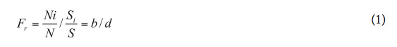
where S is the total number of pixels, N is the number of pixels with debris flow occurrences, S_i is the number of pixels of the i variable, and N_i is the number of pixels in which the debris flows occurred in the i variable (Table 1). If F_r is greater than 1, there is a high correlation; a value smaller than 1 aindicates low correlation.

Table 1.

The algorithm of logistic regression applies a maximum likelihood estimation after transforming the dependent variable into a logic variable (the natural log of the odds of the dependent occurring or not). In this manner, logistic regression estimates the probability of a certain event occurring (Atkinson and Massari, 1998) in the presence or absence of debris flows. Logistic regression is useful for predicting the presence (1) or absence (0) of a process based on a set of predictive variables. The advantages of logistic regression are that 1) each variable used can be either continuous or discrete, and 2) there is not necessarily a normal distribution.

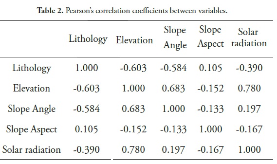
In the present situation, the binary dependent variable represents the presence or absence of debris flows. In a logistic regression analysis, it is preferable that the number of pixels representing areas with or without a process should be the same (e.g., Süzen and Doyuran, 2004; Ayalew and Yamagishi, 2005; Nefeslioglu et al., 2008); therefore, 10000 pixels representing the occurrence of debris flows and 10000 pixels without debris flows were randomly selected for logistic regression. The lithologic unit classes were considered to be categorical variables, whereas slope, elevation and solar radiation were considered to be continuous variables. Because semantically distinct parameters may have a strong correlation, the Pearson correlation coefficient was used to check the correlations between variables.

Finally, the susceptibility maps were verified and compared using known debris flow locations that were randomly selected and had not been previously used in the calculation of the models.

Results and discussion

The variables were converted to a raster grid with 15×15 m cells for the application of the logistic regression and frequency ratio models. The grid area was 3271 rows by 5144 columns (i.e., the total number is 9670614), and 155058 cells had debris flow occurrences. A total of 346 debris flows were identified (Figure 1) and covered an area of 42.45 km², accounting for 1.95% of the study area (2175.9 km²). Only 214 debris flows were used for susceptibility analysis; the rest were reserved for verification purposes.

On Table 1, the debris flow percentages that were used for the susceptibility analysis are shown, whileand the percentage distribution of all debris flows within each conditioning factor are presented in Figure 3. The Pearson correlations (Table 2) show that the variables used in the present study are only weakly correlated with each other. The highest correlation was found between solar radiation and elevation (0.78).

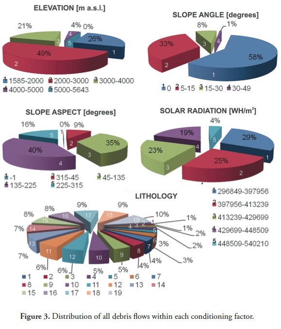
In the study area, the outcropping lithologies were grouped into nineteen classes: 1- lower Ordovician sedimentary rocks, 2- Devonian conglomerates, sandstones and pelites, 3,4,5 and 6- carboniferous marine formations, 7, 10 and 11- granites, 8- granodiorites, 9- rhyolites, 12- mesosilicic and silicic volcanic and igneous complex, 13- multicolor tuff, 14- Miocene intrusive rocks, 15- Miocene argillites, 16 and 17- Pleistocene deposits, 18- silt, and 19- recent deposits. (Figure 2). The Pleistocene deposits, which represent 40% of the total area of the studied territory, are involved in more than 44% of the total area of debris flows identified (Figure 3).

The elevation map (Figure 2) of the study area was divided into five elevation classes; the elevation ranges from 1585 to 5643 m a.s.l. A total of 72.44% of the debris flows are dominant in the elevation interval from 1585 to 3000 m a.s.l. (Figure 3).

The slope map of the study area was divided into four slope categories (Figure 2). The result shows that most of the debris flows occur at a slope angle less than 15° (Figure 3).

Aspect regions were classified according to the aspect class as flat (−1°), north (315°–360°, 0°–45°), east (45°–135°), south (135°–225°) and west (225°–315°). This factor indicates that debris flows occur on east-facing (30.19%) and south-facing (43.23%) slopes (Figure 3).

The solar radiation map indicates that debris flows occur in almost all classes with similar percentages (Figure 3).

The observed distribution of the debris flows, the frequency ratio and the logistic regression coefficients are shown in Table 1.

According to the logistic regression method, the aspect coefficient is positive, while the elevation, slope, and solar radiation coefficients are negative. This means that the aspect is positively related to the occurrence of debris flows, whereas elevation, slope, and solar radiation have an inverse relationship with debris flow occurrence in the study area. The variables chosen and the system constructed were found to be valid; 70.4% of the pixels were correctly predicted (76.7% of the pixels of the debris flows and 64.1% of the pixels of non-debris flows). Furthermore, the logistic regression analysis revealed that the distributions of the debris flows are mainly controlled by lithology and slope, as 82.1% and 75.7%, respectively, of the pixels with debris flows beingwere correctly classified.

The frequency ratios of each variable's type or class were added to calculate the debris flow susceptibility index (DFSI), according to equation 2:

DFSI = LITHOLOGYr + ELEVATIONr + SLOPEr + ASPECTr + SOLAR RADIATIONr (where, LITHOLOGYr is the frequency ratio of lithology, ELEVATIONr is the frequency ratio of elevation, SLOPEr is the frequency ratio of slope, ASPECTr is the frequency ratio of aspect, and SOLAR RADIATIONr is the frequency ratio of solar radiation) (2)

A logistic regression formula was created, as shown in equation 3, from Table 1 data:

z = LITHOLOGYb + (-0.0002 x ELEVATION) + (0.001 x ASPECT) + (-0.087 x SLOPE) + (-0.005 x SOLAR RADIATION) + z (3)

(where, ELEVATION is the elevation value, SLOPE is the slope value, ASPECTr is the aspect value, SOLAR RADIATIONr is the solar radiation;, and LITHOLOGYb are the logistic regression coefficient values listed in Table 1. z = 2.333 and is a value determined by the program).

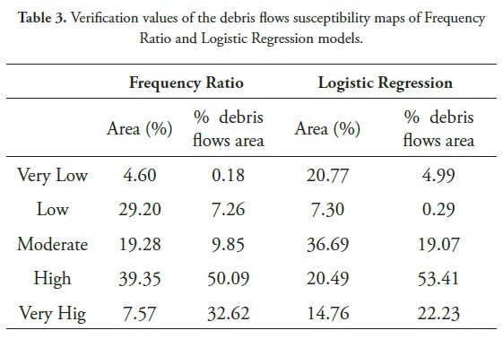
According to the debris flow susceptibility map produced from the frequency ratio method, 4.60% of the total area was haveshowed very low debris flow susceptibility. Low, moderate, high and very high susceptible zones represent 29.20%, 19.28%, 39.35% and 7.57% of the total area, respectively (Figure 4).

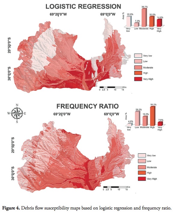
The logistic regression method showed different results with very low, low, moderate, high and very high susceptibility zones representing 20.77%, 7.30%, 36.69%, 20.49% and 14.74% of the total area, respectively.

The testing validation performed by comparing the known debris flow location data, which were not included in the susceptibility analyses, is shown in Table 3. As a result, the frequency ratio model (accuracy of 82.71%) is better for prediction than the logistic regression model (accuracy of 75.64%) for the high and very high susceptibility zones.

The precision of the susceptibility maps produced here is related to correct identification of the debris flows on the field, the interpretation of digital images and DEM resolution (90 m) with itsrespect to the derived variables (slope angle, slope aspect and solar radiation). For the method to be generally applicable, more high quality debris flow-related digital variables are necessary (DEM of major resolution of approximately 5 or 10 m). However, the susceptibility maps produced were positively tested on January 23, 2010 at 19:00, when a sizeable debris flow affected the town of Malimán de Arriba as a result of heavy rainfall. Several homes were damaged and most of the crops and farm animals were lost due to flash flooding. This validates the applicability of the methods used because the total area affected was located on high and very high susceptibility zones.

Conclusions

In this study, the frequency ratio and logistic regression models were applied to generate debris flow susceptibility maps, using the same conditioning factor database. Through fieldwork, aerial photographs, and digital satellite image interpretation, a debris flow inventory map was created. Of the 346 debris flows identified, 214 locations were used for model training, and the remaining 132 cases were used for model validation.

The logistic regression method revealed that the most important conditioning factor was lithology, and the rate of success was 82.1%. The validation results show that the frequency ratio model has an a improved prediction accuracy of 82.71%, which is better than that for the logistic regression model (82.71%). Thus, the results of the frequency ratio model showed the best prediction accuracy in debris flow susceptibility mapping.

The results and findings of the present study can help developers, planners, contractors and engineers in land-use planning and increase understanding of the occurrence and susceptibility of debris flows in the Andes and PreAndes of San Juan. Furthermore, the methodology presented here is easy to reproduce and may be applied to other mountainous regions with similar conditions. However, the models should be used cautiously for specific site development because of the scale of the analysis. Therefore, the models used in the study are valid for general planning and assessment purpose but may be less useful at the site-specific scale, where local geological and geographic heterogeneities may prevail.

Acknowledgements

This research was funded by a grant from the CONICET (National Council of Scientific and Technological Research).

References

Allmendinger, R.W., Figueroa, D., Snyder, D., Beer, J., Mpodozis, C. and Isacks, B.L. (1990). Foreland shortening and crustal balancing in the Andes at 30°S latitude, Tectonics. 9, no. 4, 789-809.         [ Links ]

Atkinson, P.M. and Massari, R. (1998). Generalized linear modeling of susceptibility to landsliding in the central Apennines, Italy, Computers and Geosciences. 24, 373–385.         [ Links ]

Ayalew, L. and Yamagishi, H. (2005). The application of GIS-based logistic regression for landslide susceptibility mapping in the Kakuda–Yahiko Mountains, Central Japan, Geomorphology. 65, no. 1-2, 15–31.         [ Links ]

Bai, S.B., Wang, J., Lü, G.N., Zhou, P.G., Hou, S.S. and Xu, S,N, (2010), GIS-based logistic regression for landslide susceptibility mapping of the Zhongxian segment in the Three Gorges area, China, Geomorphology. 115, 23–31.         [ Links ]

Bai, S.B., Wang, J., Zhou, P.G. and Ding, L. (2011). GIS-based rare events logistic regression for landslide-susceptibility mapping of Lianyungang, China, Environmental Earth Sciences. 62, no. 1, 139-149.         [ Links ]

Bonham Carter, G.F. (1994). Geographic Information Systems for Geoscientists, Modeling with GIS, Pergamon Press, Oxford, 398 pp.         [ Links ]

Brabb, E.E. (1984). Innovative approaches to landslide hazard and risk mapping. Proc., Fourth International Symposium on Landslides, vol. 1, Canadian Geotechnical Society, Toronto, Canada, 307–324.         [ Links ]

Chauhan, S., Sharma, M. and Arora, M.K. (2010). Landslide susceptibility zonation of the Chamoli region, Garhwal Himalayas, using logistic regression model, Landslides. 7, no. 4, 411-423.         [ Links ]

Das, I., Sahoo, S., Van Westen, C., Stein, A. and Hack, R. (2010). Landslide susceptibility assessment using logistic regression and its comparison with a rock mass classification system, along a road section in the northern Himalayas (India), Geomorphology. 114, no. 4, 627–637.         [ Links ]

Ercanoglu, M. and Temiz, F.A. (2011). Application of logistic regression and fuzzy operators to landslide susceptibility assessment in Azdavay (Kastamonu, Turkey), Environmental Earth Sciences. doi:10.1007/s12665-011-0912-4.         [ Links ]

Esper Angillieri, M.Y. (2010). Peligros Geológicos Asociados a Procesos de Remoción en Masa e Inundaciones con Características Destructivas. Área de Amortiguación del Parque Nacional San Guillermo. Provincia de San Juan, Ph.D. Thesis, Universidad Nacional de San Juan, Argentina, 235 pp.         [ Links ]

Fauqué, L., Cortés, J.M., Folguera, A. and Etchverría, M. (2000) .Avalanchas de rocas asociadas a neotectónica en el valle del río Mendoza, al sur de Uspallata, Revista Asociación Geológica Argentina. 55, no. 4, 419–423.         [ Links ]

Fernández, D.S. (2005). The giant paleolandslide deposits of Tafí del Valle, Tucumán Province, Argentina, Geomorphology. 70, 97– 111.         [ Links ]

Fu, P. and Rich, P.M. (2002). A geometric solar radiation model with applications in agriculture and forestry, Computers and Electronics in Agriculture. 37, 25–35.         [ Links ]

González Díaz, E.F. (2009). Deslizamientos al norte de la población de Tricao Malal, noroeste de Neuquén, Revista de la Asociación Geológica Argentina. 65, no. 3, 545-550.         [ Links ]

González Díaz, E.F. and Folguera, A. (2009). Los deslizamientos de la cordillera neuquina al sur de los 38° S: su inducción, Revista de la Asociación Geológica Argentina. 64, no. 4, 569-585.         [ Links ]

Kincal, C., Akgun, A. and Koca, M. (2009). Landslide susceptibility assessment in the Izmir (West Anatolia, Turkey) city center and its near vicinity by the logistic regression method, Environmental Earth Sciences. 59, 745–756.         [ Links ]

Lee, S. (2005). Application of logistic regression model and its validation for landslide susceptibility mapping using GIS and remote sensing data, International Journal of Remote Sensing. 26, 1477–1491.         [ Links ]

Lee, S. and Sambath, T. (2006). Landslide susceptibility mapping in the Damrei Romel area, Cambodia using frequency ratio and logistic regression models, Environmental Geology. 50, 847–855.         [ Links ]

Lee, S. and Pradhan, B. (2007). Landslide hazard mapping at Selangor, Malaysia using frequency ratio and logistic regression models, Landslides. 4, 33–41.         [ Links ]

Minetti, J.L. (1986). El régimen de precipitaciones de San Juan y su entorno. CIRSAJ-CONICET- UNSJ, Informe técnico 8, San Juan, 19-22.         [ Links ]

Moreiras, S.M. (2006). Frequency of debris flows and rockfall along the Mendoza river valley (Central Andes), Argentina, Quaternary International. 158, 110-121.         [ Links ]

Nandi, A. and Shakoor, A. (2010). A GIS-based landslide susceptibility evaluation using bivariate and multivariate statistical analyses, Engineering Geology. 110, no. 1–2, 11–20.         [ Links ]

Nefeslioglu, H.A., Duman, T.Y. and Durmaz, S. (2008). Landslide susceptibilitymapping for a part of tectonic Kelkit Valley (Eastern Black Sea region of Turkey), Geomorphology. 94, 410–418.         [ Links ]

Oh, H. and Lee, S. (2010). Cross-validation of logistic regression model for landslide susceptibility mapping at Ganeoung areas, Korea, Disaster Advances. 3, no. 2, 44–55.         [ Links ]

Perucca, L.P and Esper Angillieri, M.Y. (2008.) La avalancha de rocas Las Majaditas. Caracterización geométrica y posible relación con eventos paleosísmicos. Precordillera de San Juan, Argentina, Revista Española de la Sociedad Geológica de España. 21, no. 1-2, 35 – 47.         [ Links ]

Perucca, L.P. and Esper Angillieri, M.Y. (2009a). El deslizamiento de rocas y detritos sobre el río Santa Cruz y el aluvión resultante por el colapso del dique natural, Andes Centrales de San Juan, Revista de la Asociación Geológica Argentina. 65, no. 3, 571 – 585.         [ Links ]

Perucca, L.P. and Esper Angillieri, M.Y. (2009b). Evolution of a debris-rock slide causing a natural dam: the flash flood of Río Santa Cruz, Province of San Juan—November 12, 2005, Natural Hazards. 50, no. 2, 305-320.         [ Links ]

Penna, I.M., Hermanns, R.L. and Folguera, A. (2008). Remoción en masa y colapso catastrófico de diques naturales generados en el frente orogénico andino (36º-38ºS). Los casos Navarrete y Carrilaufquen, Revista de la Asociación Geológica Argentina. 63, no. 2, 172-180.         [ Links ]

Ramos, V.A. (1999). Las provincias geológicas del territorio argentino. R. Caminos (Editor), Geología Argentina, Anales 29, no. 3, SEGEMAR, Buenos Aires, 41–96.         [ Links ]

Rich, P.M. and Fu, P. (2000). Topoclimatic habitat models, Proceedings of the Fourth International Conference on Integrating GIS and Environmental Modeling. Alberta, Canada, 96, 1–14.         [ Links ]

Rich, P.M., Dubayah, R., Hetrick, W.A. and Saving, S.C. (1994). Using Viewshed models to calculate intercepted solar radiation: applications in ecology, American Society for Photogrammetry and Remote Sensing Technical Papers. 524–529.         [ Links ]

Süzen, M.L. and Doyuran, V. (2004). Data driven bivariate landslide susceptibility assessment using Geographical Information Systems: a method and application to Asarsuyu catchment, Turkey, Engineering Geology. 71, 303–321.         [ Links ]

Takahashi, T. (2007). Debris flow Mechanics, Prediction and Countermeasures, Taylor & Francis Group, London, UK, 448 pp.         [ Links ]

USGS. (2000). Shuttle Radar Topography Mission, 3 Arc Second. Global Land Cover Facility. InUniversity of Maryland, College Park, Maryland.         [ Links ]

Varnes, D.J. (1978). Slope movement types and processes. R.L. Schuster and R.L. Krizek (Editors.), Landslides: Analysis and Control, Special Report, vol. 176, Transportation Research Board, National Academy of Sciences, Washington, DC, 11–33.         [ Links ]

Yalcin, A., Reis, S., Aydinoglu, A.C. and Yomralioglu, T. (2011). A GIS-based comparative study of frequency ratio, analytical hierarchy process, bivariate statistics and logistics regression methods for landslide susceptibility mapping in Trabzon, NE Turkey, Catena. 85, 274–287.         [ Links ]