


Serviços Personalizados
Journal
Artigo
 Inglês (pdf)
 Artigo em XML
 Referências do artigo
 Enviar este artigo por email
Indicadores
-
 Citado por SciELO
 -
 Acessos
Links relacionados
-
 Citado por Google
 -
 Similares em
SciELO
Similares em
SciELO -
 Similares em Google
Compartilhar

 Permalink
Earth Sciences Research Journal
versão impressa ISSN 1794-6190
Earth Sci. Res. J. vol.18 no.2 Bogotá jul./dez. 2014
http://dx.doi.org/10.15446/esrj.v18n2.39716
Caving Depth Classification by Feature Extraction in Cuttings Images
Laura Viviana Galvis C.1,3, Reinel Corzo Rueda2, Henry Arguello Fuentes3
1 Grupo de Investigación Estabilidad de Pozo (GIEP). Universidad Industrial de Santander, Bucaramanga, Colombia.
2 ECOPETROL-Instituto Colombiano del Petróleo. Grupo de Investigación Estabilidad de Pozo, Piedecuesta, Colombia.
3 Escuela Ingeniería de Sistemas e Informática. Universidad Industrial de Santander, Bucaramanga, Colombia.
Record
Manuscript received: 31/08/2013 Accepted for publication: 25/09/2014
ABSTRACT
The estimation of caving depth is of particular interest in the oil industry. During the drilling process, the rock classification problem is studied to analyze the concentration of cuttings at the vibrating shale shakers through the classification of caving images. To date, depth estimation based on caving rock images has not been treated in the literature. This paper presents a new depth caving estimation system based on the classification of caving images through feature extraction. To extract the texture descriptors, the cutting images are first mapped on a common space where they can be easily compared. Then, textural features are obtained by applying a multi-scale and multi-orientation approach through the use of Gabor transformations. Two different depth classifiers are developed; the first separates the textural features by using a soft decision based on the Euclidean distance, and the second performs a hard decision classification by applying a thresholding procedure. A detailed mathematical formulation of the developed classifiers is presented.
The developed estimation system is verified using real data from rock cutting images in petroleum wells. Several simulations illustrate the performance of the proposed model using real images from a wellbore in a Colombian basin. The correct classification rate of a database containing 17 depth estimates is 91.2%.
Key words: Caving classification. Cuttings. Wellbore. Rock images. Caving depth.
RESUMEN
La estimación de la profundidad de la que provienen los derrumbes que usualmente se presentan en las caras del pozo o también llamados cavings es de gran interés en la industria petrolera. Durante el proceso de perforación de un pozo, el problema de clasificación de rocas ha sido estudiado con el fin de analizar la concentración de recortes o ripios de perforación en las zarandas vibratorias a través de la clasificación de imágenes de cavings. Sin embargo, la estimación de la profundidad de los derrumbes basada en la utilización de imágenes de los mismos no ha sido tratada en la literatura. Este artículo presenta un nuevo modelo para la estimación de la profundidad de derrumbes a través de extracción de características. Para la extracción de estas características o descriptores de textura, imágenes de recortes son transformadas en un espacio común, el cual permite su comparación. Luego, las características se obtienen aplicando la transformación de Gabor, un enfoque que se caracteriza por proporcionar un análisis multi-escala y multi-orientación. Se desarrollaron dos clasificadores, el primero separa las características de textura usando un enfoque basado en la norma Euclideana y el segundo basado en decisiones por umbral. La formulación matemática detallada de los clasificadores desarrollados se presenta en este artículo.
El sistema de estimación desarrollado se evalúa usando datos reales de imágenes de derrumbes pertenecientes a un pozo petrolero. Simulaciones muestran el rendimiento del modelo propuesto usandágenes reales de un pozo perteneciente a una cuenca Colombiana. La correcta clasificación para una base de datos de imágenes que contiene 17 clases o profundidades es de 91.2%.
Palabras clave: Clasificación de cavings. Ripios de perforación. Pozo petrolero. Imágenes de roca. Profundidad de derrumbes.
1. Introduction
A crucial problem in the oil industry is the collapse of the wellbore during the drilling process. The collapse of the wellbore occurs when pieces of rock fall from the walls of the borehole, which is usually known as caving (Aldred, et al., 1999). The costs associated with the drilling process are in the millions, and between 15% and 30% of the total resources dedicated to an oil project are designated to cover losses, including material and drilling equipment and continuity of the drilling process; these losses are known as non-productive time (Aldred, et al., 1999). Hence, classifying the rocks associated with the collapse of the wellbore is an important area of research in this industry.
In the oil industry, the estimation of the caving depth is of particular interest. Conventional techniques used in geology do not solve this problem because they require excessive processing time. Specifically, the geological age of the caving materials provides information about their approximate depth. However, this method requires a micro-paleontological analysis that is not immediately available (Aldred, et al., 1999). Despite extensive work in pattern recognition and rock classification (Crida & de Jager, 1996), (Mengko, Susilowati, Mengko, & Leksono, 2000), (Thompson, Niekum, Smith, & Wettergreen, 2005), (Wang & Lin, 2005), (Galvis, Ochoa, Arguello, Carvajal, & Calderón, 2011), (Marmo, Amodio, Tagliaferri, Ferreri, & Longo, 2005), (Bajwa & Choudhary, 2006), (Kachanuban & Udomhunsakul, 2007), research regarding depth estimation based on caving rock images is extremely limited.
The problem of rock classification during the drilling process is investigated by analyzing the cutting concentration at the vibrating shale shakers by classifying caving images (Marana, et al., 2009). The detection of a high caving concentration indicates problems such as the collapse of the well borehole walls (Castillo & Moos, 2000). The cutting concentration has been addressed using several supervised classifiers, such as the Optimum-Path Forest (OPF), Artificial Neural Networks with Multi Layer Perceptron (ANN-MLP), Support Vector Machines (SVM) and Bayesian Classifiers (BC) (Marana, et al., 2009). Artificial neural networks and SVM are the most used and result in up to 93.5% correct classification when the rocks texture is analyzed (Singh, Singh, Tiwary, & Sarkar, 2010), (Marmo, Amodio, Tagliaferri, Ferreri, & Longo, 2005). The OPF technique offers a lower computational complexity than other methods (Marana, et al., 2009). The Bayesian Classifier is the most traditional classification method, and its principal advantages include its simplicity, better performance when more data are available, and self-correction, which means that the result changes for different data (Islam, Wu, Ahmadi, & Sid-Ahmed). However, those classification methods have only a few well-established classes. Despite the diverse research into cutting concentration, research on depth estimation using caving images is lacking in the literature (Galvis, Arguello, & Tarazona, 2011).
This paper presents a new system for estimating caving depth based on features extracted from rock images. Given a set of textural rock features, the estimation system divides the caving depth into a set of depth ranges previously established as classes in the classification system. The depth classifier aims at separating the textural features by using a soft decision based on the Euclidean distance and a hard decision by using a threshold constant. The developed estimation system is verified using real data from rock cutting images in petroleum wells. Additionally, the system for estimating the depth of caving can be extended to other areas, such as mining, where problems associated with caving in a specific region of the wellbore can be avoided or addressed. This is the first work applying a classification system to estimate the depth of the caving. The principal contributions of this paper include the establishment of an extensive mathematical model for the rock classification problem and the verification of the developed model using images from real caving rocks.
An important set of caving rocks, called cuttings, are rocks whose depth origin is previously known. Each cutting rock image is considered a mosaic of different textural regions. To extract these textural regions, the cutting images are first mapped onto a common space where they can be easily compared. This mapping reduces the dimensionality of the images by retaining only the relevant information. A two-dimensional (2D) Gabor transformation is used to map the rock images as this transform emphasizes the textural features. Texture plays a particularly important role in the composition of natural images, and its analysis and classification are areas of continued research (Kachanuban & Udomhunsakul, 2007).
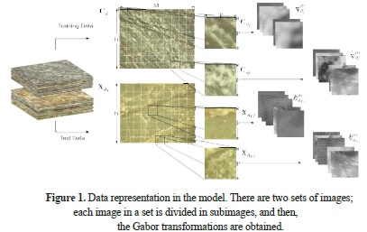
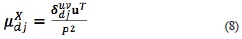
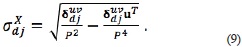
Depth classification is a multi-step process. In the first stage, a large database of rock images is acquired from a real wellbore in a Colombian basin. The sensed gray-scale images are divided into training and testing sets. The training set is denoted as C=[C1, ..., Cd, ..., CD], and the testing set is denoted as X=[Xd1, ..., XdL] where D and L indicate the number of images in each group and, traditionally, D » L. The images Cd and Xdℓ are N × M matrices representing the dth training and testing images, respectively. Figure 1 shows the representation of the data sets. The rock images in the training set belong to rocks that have a known depth d, and therefore, they are called cuttings. Conversely, images in the testing set belong to regions of caving, whose depth d must be estimated. Each image Cd and Xdℓ is again divided into H non-overlapping P x P subimages to work with small image sections and non-repeated information. The next step involves the extraction of the textural features from the training and test subsets. The selected method of texture analysis for feature extraction is critical to the success of the texture classification. A multichannel Gabor function is used for the feature extraction. This function has been recognized as a very useful tool in computer vision and image processing, especially for texture analysis (Shen, Jia, & Chen, 2011) (Clausi & Jernigan, 2000). The Gabor transformation provides a multi-scale and multi-orientation representation of the underlying images (Clausi & Jernigan, 2000). The features are extracted from the Gabor transformations and through the co-occurrence matrix (Marana, et al., 2009) (Tou, Tay, & Lau, 2009). The set of features is represented as a matrix of features FC for the training set and  X for the test set. Specifically, the κ-extracted features correspond to the mean µ, the standard deviation σ, the contrast α, the homogeneity β, the energy ɣ, and the correlation ρ.
In the classification stage, a multiclass approach is applied. In this approach, a number of binary classifiers is developed with the set of image features in the training set FC. Then, given a caving image from the test set, its set of features X is used to test the classifier. To make the decision about the class or depth to which the caving belongs, the classifier uses two methods: one method based on rules that make the decision using a hard thresholding approach and another method based on the ℓ2-norm. The number of binary classifiers depends on the number of classes or, in this case, the number of known depths D. The mathematical model for classification and the approaches presented here correctly classify depths up to 91% of the time.
The paper is organized as follows. Section 2 describes the data and process methodology, including the division of the data, the feature extraction step, the Gabor transformation used, and the classification. Section 3 presents the experimental setup. Section 4 presents the results of the simulations using data from a real wellbore in a Colombian basin.
2. Data and Methodology
Let Cd and Xdℓ be N×M matrices representing cutting and caving images, where d and dℓ represent the image depth, and let C and X be the ensemble of images Cd and Xdℓ, respectively. Thus, C=[C1, ..., Cd, ..., CD] and X=[Xd1, ..., Xdℓ, ..., XdL]. Note that C represents the training image set, X represents the test image set, and D is the number of depths. These values are associated with the number of classes in the system. Note also that C1 is the image from the first depth and that Cd is the image from the depth d.
The images Cd and Xdℓ are divided into H non-overlapping P×P subimages, such that H={h1}{h2}, where h1=[N/P] and h2=[M/P]. The jth subimage of Cd is denoted by Cdj, and the jth subimage of Xdℓ is denoted by Xdℓj. The image Cd can be expressed as a function of its subimages: Cd=[Cd1, Cd2, ..., Cdh]. Similarly, the image Xdℓ can be expressed as a function of its subimages: Xdℓ=[Xdℓ1, ..., XdℓH]. Figure 1 shows this representation of the data sets.
Let cdj and xdℓj be the vector representations of Cdj and Xdℓj, such that cdj = Vec(Cdj) and xdℓj = Vec(Xdℓj). More specifically, the vector representation of the jth subimage is given by (cdj)ℓ = (Cdj) (ℓ-rP)r' for ℓ = 0, ..., P2 - 1 and r = [ℓ-P].
2.1. Gabor Representation
The vectorscdj and xdℓj are first transformed to extract their texture features. A two-dimensional Gabor function is used because it provides a multi-scale and multi-orientation representation of the underlying signals (Clausi & Jernigan, 2000). In the spatial domain, a 2D Gabor function is a sinusoidal plane wave modulated by a Gaussian function. More specifically, the 2D Gabor function is given by
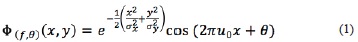
where u0 is the frequency and θ is the anti-clockwise rotation of the Gaussian function and the plane wave. The values σx and σy represent the size of the Gaussian function or the scale in the x and y dimensions, respectively.
The Gabor function in (1) can be expressed in matrix notation as:
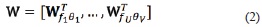
where Wfu θv represents the Gabor filter bank at frequency u and rotation v.
Using W, a discrete set of transformations is obtained. This set with different frequencies and orientations is used to extract features from the subimages. Selection of the frequencies emphasizes the intermediate frequency band as the most significant information about a texture often appears in the middle frequency channels (Zhang, Tan, & Ma, 2002), (Chang & Kuo, 1993). The frequencies are given by
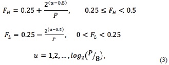
where the set of frequencies is fu = { FL, FH } and P is the size of the subimages. However, the literature indicates that a finer quantization of orientation (larger number of rotations) is needed. The restriction on the decision about the number V of rotations, θ, is based on the computational efficiency.
Given a training vectorcdj, the respective training Gabor transformation  can be written in matrix notation as
where u and v indicate the frequency and the rotation, respectively.
Analogously, the Gabor transformation of the test vectors xdℓj can be written as
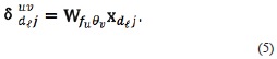
Figure 1 shows the representation of the data sets and the process used to obtain the respective transformations.
2.2. Feature Extraction
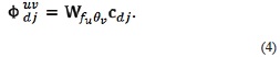
Two features, the mean  and the standard deviation
  of the classification system, can be directly estimated using the Gabor transformation in (4) and (5); the index C represents the set of images to which the transformation belongs. These features are calculated for each subimage of the training set using the transformation in (4) as
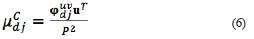
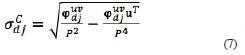
where P is the dimension of the subimage and u is a P2-long one-valued vector. Equivalently, the mean and standard deviation are calculated for the test images by using the respective in  (5) as
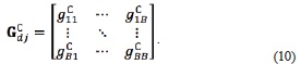
The energy, contrast, homogeneity and correlation are also calculated for the subimages, in addition to the mean and the standard deviation given in (6), (7), (8) and (9). The co-occurrence matrix is defined as a matrix or distribution of co-occurring values at a given offset. The use of this matrix is based on the assumption that the texture information on the image vector  or is contained in the overall or average spatial relationships of these vectors (Haralick, Shanmugan, & Dinstein, 1973). The co-occurrence matrix is defined as G = Q () where Q is an operator that defines the position of two pixels relative to each other. Let the elements of G be gij. Then, gij represents the number of times that pixel pairs with intensities i and j are present in an image in the position specified by Q.
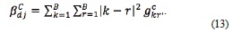
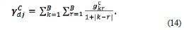
The size of this co-occurrence matrix is determined by the number of possible intensity levels in the image. For an 8-bit (256 possible levels) image, G will be 256x256. To reduce computation load, a frequently used approach is to quantize the intensities into a few bands to keep the size of the matrix G treatable. In the case of the 256 intensities, a quantization on B levels, where L = 8 results in a co-occurrence matrix of size B x B (Gonzalez & Woods, 2008). The co-occurrence matrix associated with the training image vector is given by
Accordingly, the co-occurrence matrix for the image vector is

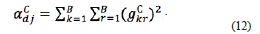
Using the co-occurrence matrices, the energy, contrast, homogeneity and correlation are calculated. The angular second moment or energy  for the training set is calculated by
The contrast or the measure of the amount of local variation  is given by
The direct measure of the local homogeneity  is calculated by
Finally, the correlation or the measure of linear dependency ρ of neighboring image pixels is given by
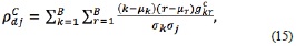
where µk, µr, σk and σr are the means and standard deviations of  and
and  , respectively.
Similarly, textural features are calculated for the testing image vector .
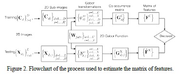
The 6 characteristics for the training set in (6), (7) and (12)-(15) are combined into the matrix FC shown in equation (16) for the H sub-images and the UV Gabor transformations of each of those sub-images. Similarly, the matrix X is constructed using the characteristics for the testing set. The columns of this matrix represent the H subimages, and the rows represent the filtered images UV for each of the k features. A flowchart of the procedure used to obtain the matrix of features of any image and to make a final decision about its classification is presented in Figure 2.
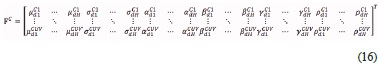
The matrices of features FC and X represent the texture at determined frequencies U and orientations V after filtering by the Gabor transformation. Some of the frequency-orientation combinations will be more representative than others, taking into account that the real frequency-rotation of the texture is adjusted to the combination given by the Gabor function.
The analysis of the data allows an image to be characterized using only a small set of the images filtered by Gabor filters. Thus, a portion of the data extracted from and can be used for the classification while the other portion is noise, making the classification more difficult. For this reason, a classification based on distances is used in this model, following heuristic rules to use the most representative features. Two approaches for the estimation of the depth d by the classification of a caving are proposed.
2.3. Classification based on a hard thresholding
In this approach, the goal is to find the subset of feature vectors that determines the texture of an image. Each feature matrix of the training classes is compared with the feature matrix of a test image. A sum of the differences of the matrices for small distances is calculated. To calculate those distances and to make a decision related to the similarity among vectors, a threshold is included in the model. This threshold τ is estimated using the training set of images. The distances in this approach are given by:
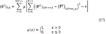
for h = 0, ..., H ‒ 1; ℓ = 0, ..., UVH ‒ 1 and  .
.
Then, the maximum value for similar features present in  is used for the classification, and this selection can be represented as
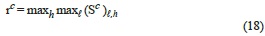
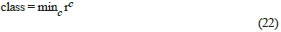
To make the decision, the training set class with the greater number of similar feature sets is established as the class to which the test image belongs. This decision is given by the comparison among the rC of the possible classes and is defined as:
2.4. Classification based on the Euclidean Norm (ℓ2)
Instead of the sum presented with the previous approach, this method uses the distances between vectors. To calculate those distances, is calculated as:

for h = 0, ..., H ‒ 1; ℓ = 0, ..., UVH ‒ 1 and .
The matrix contains the minimum distances between the features in the training and test images, and those minimum distances characterize each subimage and image, respectively. To use the most representative distances, a distance per class is obtained by

For comparison among classes, the distances between the classes are evaluated and the class with the minimum distance is selected as the class to which the test image belongs. This decision is given by the evaluation of the distances rC as:
Finally, weight can be applied in the model to give more importance to some of the features. To apply this weight, a vector ω with the weights is applied to the feature vector before the comparisons in equations (17) and (20). Then, the vector ω can be expressed as a function of the weights, ω = [ω1, ..., ωk].
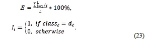
Given the images of the test set, the accuracy of each of the approaches is calculated as the sum of the successful classifications over the number of evaluations, which consists of the evaluation of the L images in the test set in this case. The equations for the calculation of the performance are
3. Experimental setup
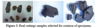
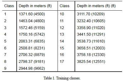
To evaluate the efficiency of the presented model, rock samples extracted from a wellbore in a Colombian basin were used. Cuttings from depths between 1371.6 and 3825.54 meters (4500-12550 ft) were acquired via real-time monitoring by the Colombian Petroleum Institute (ICP). To facilitate the process of acquisition and reduce uncertainty, specimens were created in an ICP laboratory containing samples of cuttings and caving materials. Images of some samples are presented in Figure 3.
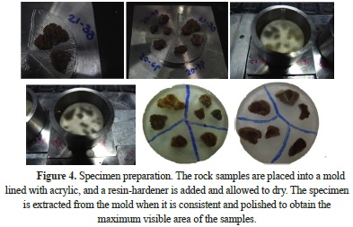
For the preparation of the specimens, the rock samples were placed in a metallic mold lined with vacuum grease or acrylic. A mixture of resin and hardening in a ratio of 1 to 2 grams was added and allowed to dry. When the specimen was completely hardened, it was extracted from the mold. Finally, the surface was polished until the visible area of the sample surface was maximized. Figure 4 shows the process used to generate specimens.
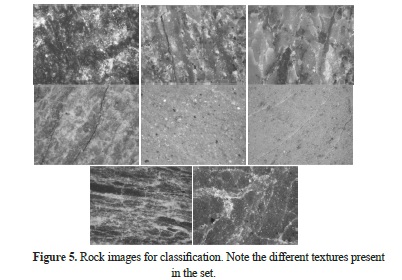
A set of images was acquired using a reflected-light microscope. Figure 5 presents some of these images, and it should be noted that different textures are present. Training set C and testing set X were thus randomly created. To simulate the classification process, a set of D = 17 classes was chosen, each representing a depth in a well as illustrated in Table 1. Then, the mathematical model presented in section 2 was applied.
A subsection of each of the images in C and X was extracted to eliminate the blurred borders that were present. Then, each image Cd and Xdℓ was divided into 12 non-overlapping subimages.
The preprocessing was performed using a bank of Gabor filters W, as presented in equation (2). For each subimage of Cd and Xdℓ, a set of U = 14 frequencies and V=6 rotations were applied, for a total of UV = 84 Gabor filters.
For each of the transformations and , k = 6 texture descriptors were calculated. An analysis of the descriptors among the different D classes allowed determining the difficulty of separation. This is the main reason to use this approach instead of traditional classification methods, given that the classes are not linearly separable. To show the non-separable characteristic, the following figures present the histograms and some examples of the features. The histograms in Figure 6 show the concentration of the descriptors in the same value ranges for two randomly selected classes. It is important to clarify that the domain does not significantly change between classes and that the overlapping behavior is similar for any pair of selected classes.
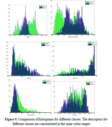
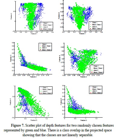
Figure 7 shows samples of two randomly selected features from the data set, and again, the overlap is similar for any pair of selected classes. Each data point is labeled according to the classes it belongs to. Here, the classes are depicted in green and blue, and the goal is to use these data as a training set to classify a new observation according to the feature classes. Note that class overlap is present in the projected space.
In evaluating the computational complexity of the algorithms, we consider two stages: feature extraction and classification. The two stages can be performed efficiently, requiring Ơ(UVH + D2) operations per image, where H is the number of subimages (12 in our experiments), U and V are the frequency and rotation of the Gabor filter bank, respectively, and D is the number of classes.
4. Simulations and results
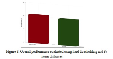
The classification was performed following the mathematical model in section 2. To calculate the performance of this method, the correct classification of each of the binary classifiers must be considered. The general performance calculated using equation (23) for each of the approaches—hard thresholding and ℓ2 -norm—is presented in Figure 8. The performance results obtained using real data and the two approaches are 91.3% and 87.5%, respectively, for the hard thresholding and ℓ2-norm approach.
To highlight the influence of the different features, the performance was calculated using different numbers and combinations of features. Figure 9 shows the performance using 4,5 and 6 features, and each of the bars represents a different combination of features. The comparison shows that the performance increases with the number of features and becomes more precise for k = 4,5,6. The best performance is obtained using the complete set of features.
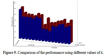
Given the variability in the performance, especially when 4 features were used, an analysis was performed to determine whether some features are dominant over the others following the weighting method in the mathematical model. Simulations involving the total number of features and assigning weights were performed by applying the vector ω. Improvements in the performance obtained using the hard thresholding classification resulted in 92%, 93% and 94% success when the weight values ω2, ω4 and ω5 were respectively applied to the standard deviation, contrast and homogeneity with greater consideration compared with the other features. The weight values considered in the analysis were ω2 = 1.2, ω4 = 1.6 and ω5 = 1.6.
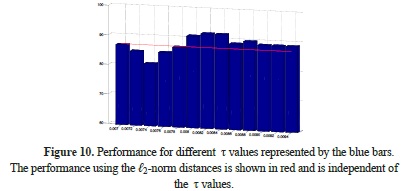
Different settings were tested in the hard thresholding classification, which includes a threshold value τ. Figure 10 shows the variation in classification accuracy for 13 different values of τ for the proposed κ features and distance measures. Figure 10 shows the independence of the performance from the ℓ2-norm distance, represented by the red line, and the best performance achieved was 91.3% correct classification using the hard thresholding approach and a τ value of 0.008.
The performance of the binary classifiers is presented in Figure 11; values of 0 (blue) above the diagonal represent classification errors and values of 1 (red) represent a successful classification. The point highlighted in Figure 11a represents a classification error in the binary classifier among classes 2 and 4 for the hard thresholding classification.
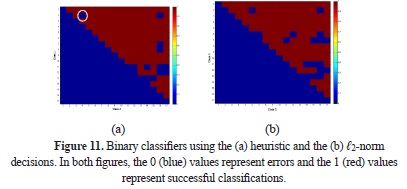
In Figure 11b, some of the classifier errors are present in binary classifiers involving the same class. For instance, the errors in classes 2 - 16, 11 - 16 and, 12 - 16 indicate that some classes as the 16 in this case present very similar features compared to other classes, which makes the classification more difficult.
Conclusions
The classification of caving depth estimation using hard thresholding and the ℓ2-norm has been developed in this work. The developed methods and a complete mathematical model are then used to classify caving depths by features extracted from cutting images. The multi-scale and multi-orientation representation obtained using Gabor filters permit a much more complex characterization of the texture due to the independence of the rotation used in the acquisition process. The performed analysis precisely extracts the texture features for different rotations, which allows an optimal comparison among the images in a training set and a testing set.
The size of the images and the number of Gabor filters applied are important because these parameters allow a complete characterization of the texture. However, as a consequence, additional information is included. This information is noise and should be removed for the classification process. The approaches in this work treat this problem by searching a reduced and a representative set. Additionally, simulations using different numbers of feature combinations reveal variation in the performance of these methods. However, none of the combinations with fewer features than the established κ achieved a greater performance.
The performance achieved with the hard thresholding classification is 91.3%, whereas the ℓ2-norm based classification achieved 87.5% success. These values demonstrate the applicability of the methods and techniques developed in this work. In addition, these methods can be applied directly in rock classification problems.
References
Aldred, W., Plumb, D., Bradford, I., Cook, J., Gholkar, V., Cousins, L., et al. (1999). Managing drilling risk. Oilfield Review, 2-19. [ Links ]
Bajwa, I. S., & Choudhary, M. A. (2006). A study for prediction of minerals in rock images using back propagation neural networks. International conference on advances in space technologies (pp. 185-189). IEEE. [ Links ]
Castillo, D. A., & Moos, D. (2000). Reservoir geomechanics applied to drilling and completion programs in challenging formations: North West shelf, Timor sea, North sea and Colombia. APPEA, 509-521. [ Links ]
Chang, T., & Kuo, C.-C. J. (1993). Texture analysis and classification with tree-structured wavelet transform. IEEE transactions on image processing, 429-441. [ Links ]
Clausi, D. A., & Jernigan, M. E. (2000). Designing Gabor filters for optimal texture separability. Pattern Recognition, 33, 1835-1849. [ Links ]
Crida, R. C., & de Jager, G. (1996). Multiscalar rock recognition using active vision. International Conference on Image Processing. 1, pp. 345-348. IEEE. [ Links ]
Galvis, L. V., Arguello, H., & Tarazona, D. (2011). Digital image processing and artificial intelligence applied to the oil wells drilling. Fuentes: el reventón energético, 21-31. [ Links ]
Galvis, L. V., Ochoa, C., Arguello, H., Carvajal, J., & Calderón, Z. H. (2011). Estimation of mechanical properties of rock using artificial intelligence. Ingeniería y Ciencia, 7 (14), 83-103. [ Links ]
Gonzalez, R. C., & Woods, R. E. (2008). Digital Image Processing (Third ed.). Pearson Prentice Hall. [ Links ]
Haralick, R. M., Shanmugan, K., & Dinstein, I. (1973). Texture Features for Image Classification. Transactions on systems, man and cybernetics, 3, 610-621. [ Links ]
Islam, M. J., Wu, Q. J., Ahmadi, M., & Sid-Ahmed, A. Investigating the performance of Naive-Bayes classifiers and K-Nearest Neighbor classifiers. International Conference on Convergence Information Technology, (pp. 1541-1546). Gyeongju. [ Links ]
Kachanuban, T., & Udomhunsakul, S. (2007). Natural rock images classification using spatial frequency measurement. International Conference on Intelligent and Advanced Systems, (pp. 815-818). [ Links ]
Marana, A. N., Chiachia, G., Guilherme, I. R., Papa, J. P., Miura, K., Ferreira, V. D., et al. (2009). An intelligent system for petroleum well drilling cutting analysis. International Conference on Adaptive and Intelligent Systems (ICAIS 2009) (pp. 37-42). IEEE. [ Links ]
Marmo, R., Amodio, S., Tagliaferri, R., Ferreri, V., & Longo, G. (2005). Textural identification of carbonate rocks by image processing and neural network: Methodology proposal and examples. Computers & Geosciences, 31 (5), 649-659. [ Links ]
Mengko, T. R., Susilowati, Y., Mengko, R., & Leksono, B. E. (2000). Digital image processing technique in rock forming minerals identification. The 2000 IEEE Asia-Pacific Conference on Circuits and Systems. (pp. 441-444). IEEE. [ Links ]
Shen, L., Jia, S., & Chen, W. (2011). Extracting local texture features for image-based coin recognition. IET Image Processing, 5 (5), 394-401. [ Links ]
Singh, N., Singh, T. N., Tiwary, A., & Sarkar, K. M. (2010). Textural identification of basaltic rock mass using image processing and neural network. Computational Geosciences, 14 (2), 301-310. [ Links ]
Thompson, D., Niekum, S., Smith, T., & Wettergreen, D. (2005). Automatic Detection and Classification of Features of Geologic interest. 2005 IEEE Aerospace Conference, (pp. 366-377). [ Links ]
Tou, J. Y., Tay, Y. H., & Lau, P. Y. (2009). Gabor Filters as Feature Images for Covariance Matrix on Texture Classification Problem. Advances in Neuro-Information Processing Lecture Notes in Computer Science, 5507, 745-751. [ Links ]
Wang, Q., & Lin, Q. (2005). Rock types detection and classification through the orthogonal subspace projection approach. International Geoscience and Remote Sensing Symposium. IGARSS. 4, pp. 2910-2913. IEEE. [ Links ]
Zhang, J., Tan, T., & Ma, L. (2002). Invariant texture segmentation via circular Gabor filters. 16th International Conference on Pattern Recognition, 901-904. [ Links ]
