


Serviços Personalizados
Journal
Artigo
 Inglês (pdf)
 Artigo em XML
 Referências do artigo
 Enviar este artigo por email
Indicadores
-
 Citado por SciELO
 -
 Acessos
Links relacionados
-
 Citado por Google
 -
 Similares em
SciELO
Similares em
SciELO -
 Similares em Google
Compartilhar

 Permalink
Earth Sciences Research Journal
versão impressa ISSN 1794-6190
Earth Sci. Res. J. vol.20 no.1 Bogotá jan./mar. 2016
https://doi.org/10.15446/esrj.v20n1.41079
http://dx.doi.org/10.15446/esrj.v20n1.41079
Shear-wave Velocity Structure of Greenland from Rayleigh-wave Analysis
Estructura de velocidad de cizalla de Groenlandia obtenida de análisis de onda Rayleigh
V. Corchete*
Higher Polytechnic School, University of Almeria, 04120 ALMERIA, Spain
* Corresponding author. Fax +34 950 015477; e-mail: corchete@ual.es
Record
Manuscript received: 05/12/2013 Accepted for publication: 30/11/2015
How to cite item
Corchete, V. (2016). Shear-wave Velocity Structure of Greenland from Rayleigh-wave Analysis. Earth Sciences Research Journal, 20(1), A1-A11. doi: http://dx.doi.org/10.15446/esrj.v20n1.41079
ABSTRACT
The elastic structure beneath Greenland is shown by means of S-velocity maps for depths ranging from zero to 350 km, determined by the regionalization and inversion of Rayleigh-wave dispersion. The traces of 50 earthquakes, occurring from 1990 to 2011, have been used to obtain Rayleigh-wave dispersion data. These earthquakes were registered by 21 seismic station located in Greenland and the surrounding area. The dispersion curves were obtained for periods between 5 and 200 s, by digital filtering with a combination of MFT (Multiple Filter Technique) and TVF (Time Variable Filtering). Later, all seismic events (and some stations) were grouped to obtain a dispersion curve for each source-station path. These dispersion curves were regionalized and inverted according to the generalized inversion theory, to obtain shear-wave velocity models for a rectangular grid of 16x20 points. The shear-velocity structure obtained through this procedure is shown in the S-velocity maps plotted for several depths. These results agree well with the geology and other geophysical results previously obtained. The obtained S-velocity models suggest the existence of lateral and vertical heterogeneity. The zones with consolidated and old structures present greater S-velocity values than the other zones, although this difference can be very little or negligible in some case. Nevertheless, in the depth range of 15 to 45 km, the different Moho depths present in the study area generate the principal variation of S-velocity. A similar behaviour is found for the depth range from 80 to 230 km, in which the lithosphere-asthenosphere boundary (LAB) generates the principal variations of S-velocity. Finally, the new and interesting feature obtained in this study: the definition of the base of the asthenosphere (for the whole study area and for depths ranging from 130 to 280 km, respectively) should be highlighted.
Keywords: Rayleigh wave, Shear wave, crust, upper mantle, Greenland.
RESUMEN
La estructura elástica bajo Groenlandia es mostrada por medio de mapas de velocidad de onda para profundidades variando desde cero a 350 km, determinada por la regionalización e inversión de la dispersión de onda Rayleigh. Las trazas de 50 terremotos, ocurridos desde 1990 hasta 2011, han sido usados para obtener datos de dispersión de onda Rayleigh. Estos terremotos fueron registrados por 21 estaciones sísmicas localizadas en Groenlandia y el área circundante. Las curvas de dispersión fueron obtenidas para periodos entre 5 y 200 s, por filtrado digital con una combinación de MFT (Técnica de Filtrado Múltiple) y TVF (Filtrado en Tiempo Variable). Después, todos los eventos sísmicos (y algunas estaciones) fueron agrupados para obtener una curva de dispersión para cada trayecto fuente-estación. Estas curvas de dispersión fueron regionalizadas e invertidas de acuerdo con la teoría de la inversión generalizada, para obtener modelos de velocidad de cizalla para una rejilla rectangular de 16x20 puntos. La estructura de velocidad de cizalla obtenida a través de este procedimiento es mostrada in los mapas de velocidad de onda S representados para varias profundidades. Estos resultados muestran buen acuerdo con la geología y con otros resultados geofísicos obtenidos previamente. Los modelos de velocidad de onda S obtenidos sugieren la existencia de heterogeneidad lateral y vertical. Las zonas con estructuras antiguas y consolidadas presentan mayores valores de velocidad de onda S que las otras zonas, aunque esta diferencia puede ser muy pequeña o despreciable en algún caso. No obstante, en el rango de profundidad de 15 a 45 km, las diferentes profundidades del Moho presentes en el área de estudio generan la principal variación de velocidad de onda S. Un comportamiento similar es encontrado para el rango de profundidad desde 80 a 230 km, en el cual la frontera litosfera-astenosfera (LAB) genera las principales variaciones de velocidad de onda S. Finalmente, debería ser destacada la nueva e interesante característica obtenida en este estudio: la definición de la base de la astenosfera (para el área de estudio completa y para profundidades variando desde 130 a 280 km, respectivamente).
Palabras clave: Onda Rayleigh, onda de cizalla, corteza, manto superior, Groenlandia.
1. Introduction
The great ability of the Rayleigh-wave dispersion analysis to delineate the Earth's deep structure is well known (Corchete, 2013a). This methodology allows the features of the Earth's structure to be determined, because it is well known that the surface-wave dispersion (Rayleigh-wave dispersion) is related to the Earth's structure crossed by the waves (represented by the S-velocity structure). Thus, the features of the elastic structure for any region of Earth can be studied through the analysis of Rayleigh-wave dispersion. In this paper, the features of the elastic structure beneath Greenland (and its surrounding area) will be revealed through this analysis.
Greenland is one of the earth regions for which there are relatively few seismic studies (it is among the most poorly studied regions of Earth), due to the particular conditions of this region (it is covered by a large and thick ice sheet), which have made difficult the development and maintenance of high-quality seismic networks. Nevertheless, since the knowledge of the crust and upper-mantle structure of this region can be the key to answer essential questions about the pre-history of Earth, the determination of a detailed seismic structure of this region could be of great importance. Fortunately, in the last years, international agencies (as GSN, IRIS and GEOFON) joint to local agencies (as Canadian, Norwegian and Danish Seismograph Networks or the international GLISN project) have been able to develop and support new and permanent broad-band digital seismic stations. As a consequence of this, in the last twenty years high-quality seismic records have been made available from seismographic databases for Greenland and its surrounding area (although the best seismic records are only available for the last 12 years).
In pioneer studies, Gregersen (1970, 1982) investigated crust structure in Greenland using surface waves. They used periods of the fundamental modes ranged from 15 to 55 s, obtaining shear-velocity profiles from 0 to 50 km of depth. These very old studies are relevant, in spite of the very limited data used. Later, Dahl-Jensen et al. (2003) provided information about the Moho depth, in many locations in Greenland, calculated from receiver-function analysis. These depths have later been confirmed by other authors as Braun et al. (2007), but they didn't perform any surface-wave tomography. The first attempt of tomography for Greenland was performed by Darbyshire et al. (2004), who investigated the crust and upper mantle structure using surface-wave tomography by first time. They used periods of the fundamental modes of Rayleigh-wave phase-velocity from 30 to 185 s, performing maps of regionalized phase velocity for some selected periods (from 30 to 146 s), but no S-velocity mapping was obtained with depth. They only performed some S-wave velocity profiles (from 50 to 350 km of depth). The lithosphere-asthenosphere boundary (LAB), inferred from these S-velocity profiles agree well with the LAB calculated by Kumar et al. (2005), from receiver-function analysis. Finally, Pilidou et al. (2005) performed a Rayleigh-wave tomography for the North Atlantic area, in which they obtained S-velocity maps from 75 to 350 km of depth (although the resolution decreases drastically with depth from 200 km). Nevertheless, in the study performed by Pilidou et al. (2005), the region of Greenland is very small in size comparing with the wide study area considered by them. As a consequence, a very poor resolution is achieved by this S-velocity mapping for Greenland and its surrounding area.
It should be noted that no 3D S-velocity structure has been obtained for Greenland and its surrounding area, for depths ranging from 0 to 75 km. Furthermore, the S-velocity structure obtained in this previous study shows a poor resolution for the depth range from 200 to 350 km. Also, it should be noted that the Greenland crust and upper-mantle structure never has been the subject of a surface-wave tomography survey, only it has been investigated as part of a bigger area (the North Atlantic region). The goal of the present study is the determination of the elastic S-velocity structure beneath Greenland and the surrounding area, from Rayleigh-wave analysis, for the whole depth range from 0 to 350 km. This Rayleigh-wave analysis will consist of filtering of Rayleigh waves, to obtain dispersion curves from 5 to 200 s.
This dispersion analysis will be performed in several steps. First, all seismic events will be grouped in source zones to get an average dispersion curve for each source-station path. Then, the dispersion curves will be obtained by digital filtering with a combination of the Multiple Filter Technique (MFT) and Time Variable Filtering (TVF). Thus, a set of source-station averaged dispersion curves will be calculated. This set of dispersion curves will be regionalized and then inverted according to the generalized inversion theory, to get S-wave velocity models for a rectangular grid defined in the study area. Finally, these models will be plotted to obtain a 2D mapping of the 3D S-wave velocity structure, for the study area. The period range to be obtained in the present study, by digital filtering, will be wider than the period range measured in the previous studies. Thus, the determination of the 3D S-velocity structure, in the whole depth range from 0 to 350 km, will be more accurate in the present study than the previous studies, in which no surface-wave dispersion was measured in the period ranges from 5 to 30 s and from 146 to 200 s.
2. Data set
In this study, 50 earthquakes occurring from 1990 to 2011 in the neighbour of Greenland have been considered (Supplement 1). These earthquakes have been registered by 21 seismic stations located in this region (Supplement 2). From these stations digital data are available recorded with a different instrument for each available channel (Supplement 6). From all these channels, only the records for the channels: BHZ, LHZ, BLZ, LLZ, BH1, LH1, BH2, LH2; have been considered as the most suitable data for this study, because the period interval of best registration for these channels is between 1 or 5 to 200 or 250 s (period interval in which the frequency response is almost flat). This period interval (from 5 to 200 s) is more suitable for exploring the elastic structure of the Earth, for a depth range of 0 to 350 km of depth.
Also, to ensure the reliability of the results, only the earthquake traces in which a well-developed Rayleigh wave train is present, with a very clear dispersion, have been considered. Thus, many records have been discarded.
The instrumental response must be taken into account to avoid the time lag introduced by the seismograph system and all distortions produced by the instrument. This correction recovers the true amplitude and phase of the ground motion, allowing the analysis of the true dispersion of Rayleigh waves. For this reason, all the traces considered in this study were corrected for instrument response.
3. Pre-processing and filtering
For the pre-processing and calculation of dispersion curves, the computation method detailed by Corchete et al. (2007) was followed. In this paper, only a brief review of the principal concepts of this methodology will be presented.
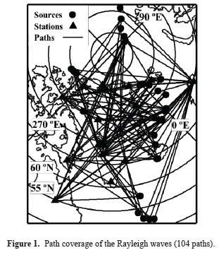
Grouping of stations and seismic events. It is well known that Rayleigh waves propagated along near epicentre-station paths show similar dispersion curves, because they cross the same earth structure and sample the same elastic properties of the medium. As a consequence of this, it is possible to group all seismic events listed in Supplement 1 in source zones, as listed in Supplement 3, to get source-station paths from epicentre-station paths. These source zones are defined as a location at which seismic events with similar epicentre coordinates have occurred. The coordinate differences for a group of events must be less than or equal to 1 degree in latitude and longitude, to be able to group them in the same source zone. Then, an average dispersion curve for each source-station path can be obtained, when the dispersion curves calculated for the traces of the events of this source zone (recorded at the same station) are averaged. In this way, any small deviations obtained are considered errors, which can be described by the standard deviation. It should be noted that some stations considered in this study also show very similar coordinates. Thus, they have been also grouped using the same criteria described above for the events, defining new station codes to denote these average stations. These new stations are listed in Supplement 4. Figure 1 shows the path coverage obtained for the study area (given by the source-station paths).
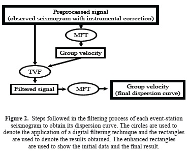
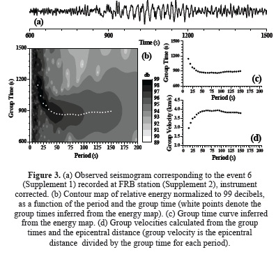
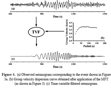
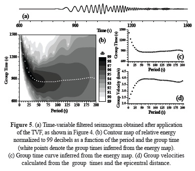
Dispersion analysis. The Rayleigh-wave group velocity for the trace of each event registered has been measured by means of the combination of digital filtering techniques: Multiple Filter Technique (Dziewonski et al., 1969) and Time Variable Filtering (Cara, 1973), as shown in the flow chart displayed in Figure 2. As an example of this filtering process, the application of this combination of filtering techniques to the trace of the event 6 (recorded at FRB station) will be detailed. The MFT (Multiple Filter Technique) has been applied firstly to this trace as it is shown in Figure 3. This trace and the dispersion curve obtained are used to compute the digital filtered signal by using the TVF (Time Variable Filtering). Figure 4 shows the time-variable filtered signal resulting from the TVF. Finally, Figure 5 shows the final dispersion curve obtained after application of the MFT to the filtered signal. A comparison between Figures 3 and 5 shows the benefits of the proposed filtering process. It should be noted that a combination of MFT and TVF works better than the application of the MFT only, because the signal/noise ratio is highly increased.
Average dispersion curves and estimation of the error. When the dispersion curves of the traces for each event involved in a source-station path have been calculated. The average group velocity for this path can be obtained as a mean of the group-velocity values calculated for each period. An estimation of the error for this media is calculated by the standard deviation (1-s error). For paths with only one event involved, a mean of the standard deviations obtained for the other near paths (which have more than one event involved) can be considered as a good estimation of the error. The average group velocities obtained for the 104 source-station paths considered in this study are listed in Supplement 5 for several periods. The periods for these dispersion curves range from 5 to 200 s. It should be noted that the period range obtained in the present study exceeds the period range obtained in previous studies (Darbyshire et al., 2004; Pilidou et al., 2005). This fact points to a better determination of the elastic structure beneath Greenland for shallow and deeper depths, if the present dispersion data are used.
4. Regionalization of group velocities
The above-described group velocities constitute the dispersion curves to be considered for regionalization. The period range of these curves goes from 5 to 200 s (Supplement 5) and there are 104 dispersion curves corresponding to the source-station paths shown in Figure 1, a dispersion curve for each source-station path. Thus, for each above-mentioned path, the forward problem in the regionalization of the surface-wave velocities is expressed as (Keilis-Borok, 1989)
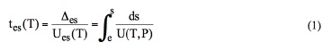
where Ues(T) is the group velocity (dispersion curve) observed between the source and the station along a great-circle path connecting those two points (the source-station path), Δes is the source-station distance (Δes =fds) and U(T, P) is the local velocity at a period T and a point P of the earth surface (on the great-circle path that connects the source and the station). The inverse problem is posed to calculate the local surface-wave velocity U(T, P), at each period T and at each point P, from the average group velocity Ues(T) previously measured for a number M of source-station paths. The inverse problem defined in these terms is known as regionalization of the surface-wave velocities. This inverse problem can be simplified, if the reciprocal of the local group velocity U(T, P), or equivalently the slowness S(Φ, λ), is firstly represented in a general stereographic polar projection (rotated 45 degrees on longitude) by the equations
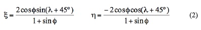
where (Φ, λ) are the geographical latitude and longitude of the point P (on the earth surface considered as a sphere). Later, S(ξ, η) is expanded into a Fourier series by the formula
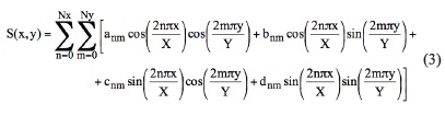
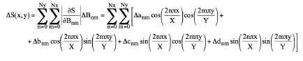
where x is ξ; - ξ0 and y is η - η0, (ξ0, η0) are the coordinates of the point at the bottom left corner of the study area (Figure 1), X is ξmax - ξ0 and Y is ηmax - η0, (ξmax, ηmax) are the coordinates of the point at the top right corner of the study area (Figure 1) and (anm, bnm, cnm, dnm, Ny and Nx) are constants. It should be noted that U(x, y) takes the velocity values of U(T, P), i. e., U(x, y) = U(Φ, λ) and S(x, y) = S(Φ, λ), for each period T, because each point P (on the earth surface considered as a sphere) has coordinates (x, y) and (Φ, λ) related by the equations (2). If formula (3) is introduced in the relationship (1) the group time can be expressed as
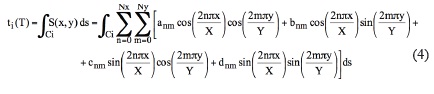
where ti is the group time of the ith source-station path (with i =1, 2, ..., M), Ci is the great-circle that connects the source and station points of the ith source-station path. It should be noted that M is the number of source-stations paths measured for the period T (104 paths maximum for this study). Equations (4) also can be written in the form
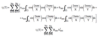
where Bnm is (anm; bnm; cnm; dnm) and
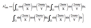
Then, equations (4) can be expressed as a system of linear equations, for each period T, in the form
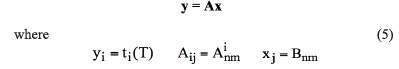
Formula (5) is a set of M linear equations, for a given period T, with N unknowns xj (with j =1, 2, N), where N = 4(Ny+1)(Nx+1). It should be noted that there is a forward problem posed for each period T, for which the equations (5) can be written. In each forward problem, the number of equations M can take different values depending on the considered period T, because the path coverage can be different for each period (Supplement 5). As a consequence of this, the number of unknowns N that can be properly determined may be also different in each problem, because always N must be less than or equals to M. Otherwise, formula (5) will be a set of equations with more unknowns N than equations M, being very difficult or impossible the determination of the unknowns xj or equivalently the Bnm coefficients of formula (3).
Once the forward problem has been defined by formula (5), for each period T, the regionalization of the surface-wave velocities is performed by the inversion of formula (5), or equivalently inverting the matrix A. The inverse matrix of A can be obtained using the inverse method detailed by Corchete and Chourak (2010). This inverse matrix is given by
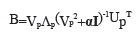
The matrix B defined by formula (6) is called the damped generalized inverse. Then, the linear equations given by formula (5) are inverted to obtain x by means of
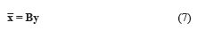
where it should be noted that

The product of matrixes B and A is called resolution matrix and it is obtained through
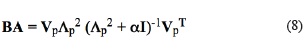
If the resolution matrix given by formula (8) is the identity matrix, the obtained solution  is unique and the resolution is perfect. Nevertheless, the addition of the factor a in the main diagonal makes that the equality Δ = I is only reached when the damping factor a is zero. The introduction of the damping parameter degrades resolution, but stabilizes the obtained solution by means of the reduction of the variance (Corchete and Chourak, 2010). The error Δ in the model parameters (or equivalently the error in the solution ) due to the error Ay in the data (i. e. the error in the group times), is given by the corresponding covariance matrix < Δ, ΔT> as (Aki and Richards, 1980)
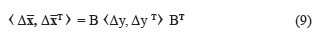
where < > indicates averaging, B is given by (6) and the covariance matrix for Δ is calculated from the covariance matrix of the error in data Δy. Assuming that all the components of the data vector y are statistically independent (or assuming an independent error for each individual measurement), i. e. assuming that the fluctuation in any data is entirely independent of the fluctuation of other data, the off diagonal elements are made zero. Then, the main diagonal elements of the data covariance matrix < Δ, ΔT >are the variances of the data. If a similar behaviour is assumed for the model parameters x (i. e. assuming that all the components of the vector x are statistically independent), the off diagonal elements are made zero. Then, the main diagonal elements of the model covariance matrix < Δ, ΔT > are the variances of the model parameters.
The obtained solution (or equivalently the set of coefficients Bnm) is calculated introducing the relation (6) in the equations (7). After, the slowness S(x, y), or equivalently its reciprocal U(x, y), is computed from these coefficients Bnm using formula (3). The errors in the model parameters (or equivalently the errors in the coefficients Bnm) are obtained by means of the relation (9). Later, the error in the slowness S(x, y) is computed from the errors in the coefficients Bnm using the partial derivative of formula (3) given by
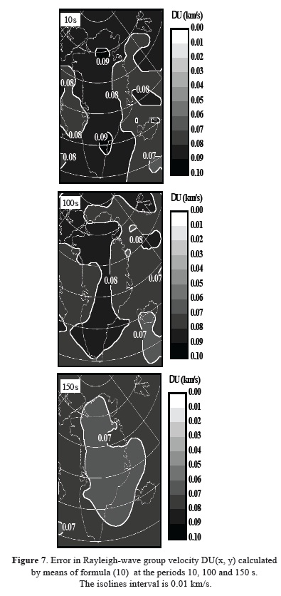
Finally, the error in the local group velocity U(x, y) is computed from
then
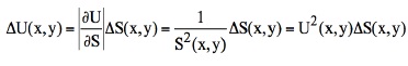
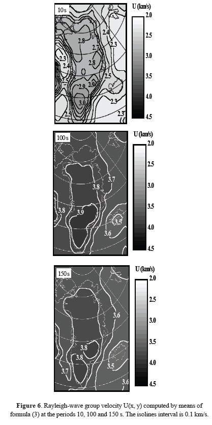
the error in the slowness S(x, y), using also the partial derivative of the formula Figure 6 shows the regionalized group velocity U(x, y) obtained following the above-described method for the periods 10, 100 and 150 s. Figure 7 shows the errors of the regionalized group velocity DU(x, y) for the same periods.
5. Inversion of regionalized dispersion curves
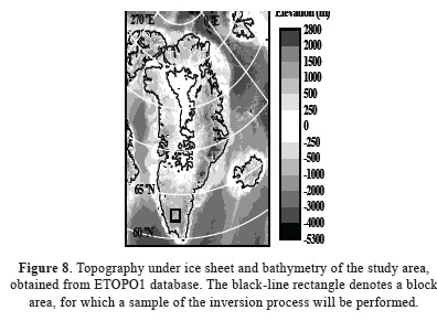
The above-described group velocity distributions with period must be inverted to obtain the shear-wave velocity distribution with depth (the 3D S-velocity structure for Greenland and its surrounding area). For it, these group velocity surfaces U(x, y) calculated for each period, from 5 to 200 s, are sampled in a rectangular grid of 16x20 points. Really, these grid points are the centres of a grid with 16x20 rectangular blocks, as the block shown in Figure 8. These grid data can be inverted obtaining a shear velocity model (a shear velocity distribution with depth) for each grid point (or block) of the study area, achieving thus a 3D S-velocity model that represents the 3D elastic structure beneath Greenland and its surrounding area. The inversion of the group velocity, for each grid point of the study area, will be performed using the computation method described in detail by Corchete et al. (2007). Here only a brief review of the principal concepts of this methodology is presented.
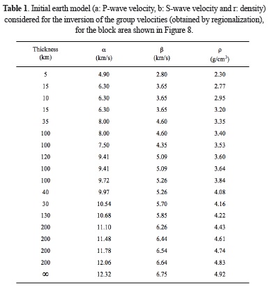
Selection of an initial earth model. The selection of an initial earth model is a preceding step before the inversion process. The initial model must be prepared considering all information available for the study area, with respect to the S-wave, P-wave and density distributions with depth. For the present study, this geophysical and geological information has been obtained from previous studies developed in the study area, which are mentioned in the introduction section of this paper. This information has been incorporated to the initial models, for the above-mentioned grid points (or blocks). Particularly, the Moho depths calculated by Dahl-Jensen et al. (2003), for many places in Greenland, has been used to provide the Moho depth in the initial models, as well as the Moho depths predicted by the Moho map performed by Braun et al. (2007). Thus, an initial model has been prepared for each grid point (or block) for depths ranging from 0 to 400 km. For depths deeper than 400 km, the PREM model developed by Dziewonski and Anderson (1981) has been used. These models must provide a theoretical dispersion curve as close as possible to the observed curve, because the inversion scheme to be used only considers small perturbations for the wave velocities involved. As an example, the initial model considered for the inversion of the dispersion curve (group velocity), associated with the grid point located at the centre of the block shown in Figure 8, is listed in Table 1 and its shear-wave velocity distribution with depth is plotted in Figure 9a (dashed line). The theoretical group velocity shown in Figure 9c (dashed line) is calculated by forward modelling, from the starting model listed in Table 1.
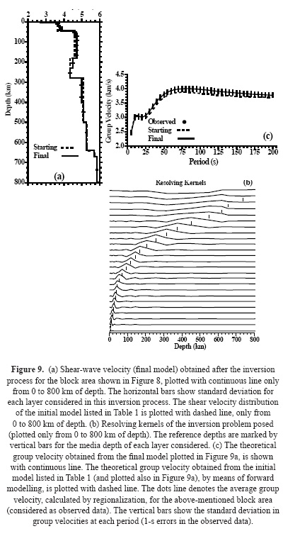
Inversion. When the starting model is ready, the group velocity can be inverted to obtain the corresponding S-velocity distribution with depth. Figure 9 show the results of an example of such inversion. In this example, the dispersion curve corresponding to the block area shown in Figure 8 has been inverted. The S-velocity model shown in Figure 9a (continuous line) is the final model obtained for this block. The model improvement iteratively obtained, is checked by the comparison between the observed group velocity (considered as observed data) and the theoretical group velocity (calculated from the actual model by forward modelling and considered as theoretical data). When the theoretical curve falls within the vertical error bars of the observed curve, as shown in Figure 9c, the inversion process is finished, because the obtained S-velocity model describes the observed curve within its experimental error.
Resolution of the final model. The resolving kernels shown in Figure 9b indicate the reliability of the solution obtained for the inverse problem posed. A good engagement between the calculated solution and the true solution (which implies the reliability of the estimated solution), is obtained when the absolute maxima of these functions fall over the reference depths. This reliability is also related to the width of these absolute maxima. The solution for the inversion problem is more reliable when the maxima of these resolving kernels are narrower. It should be noted that the S-velocity models (Figure 9a) and the resolving kernels (Figure 9b), are plotted only for depths above 800 km. This fact is due to the bad resolution obtained for depths deeper than 350 km. Figure 9b shows that the deeper layers (below 350 km) have a poor resolution. This is shown in the lack of coincidence between the resolving-kernel absolute maxima and their reference depths, for depths down to 350 km. Therefore, the results obtained for depths below 350 km have been left out, because the resolution at these deeper depths is poor. For depths of 0 to 350 km, the S-velocity models must be considered as valid models. Thus, the S-velocity final model shown in Figure 9a (continuous line), from 0 to 350 km of depth, is the definitive S-velocity distribution with depth calculated for the above-mentioned block area. This S-velocity distribution agrees well with the results obtained by Darbyshire et al. (2004), for the Greenland lithosphere. Nevertheless, this comparison only can be approximately done, because they didn't calculate S-velocity profiles in the southernmost part of Greenland. Moreover, they didn't perform S-wave velocity profiles from 0 to 50 km of depth. For it, at this depth range, it is not possible any comparison with the S-velocity profile shown in Figure 9a. This profile also can be compared with the mapping performed by Pilidou et al. (2005), for the North Atlantic area, in which the region of Greenland is included, but this region is very small in size comparing with the big size of the wide study area considered by them. As a consequence of this, a very poor resolution is achieved by this S-velocity mapping for Greenland and its surrounding area, which makes difficult the precise comparison between this mapping and the S-velocity profile shown in Figure 9a. Logically, the information about the Greenland structure that can be discerned from global mappings will have always a poor resolution. On the other hand, the S-velocities shown in Figure 9a present high values in general, as expected for the block area shown in Figure 8, which is inside of an Archean block that hosts some of the oldest rocks on Earth and therefore has a high rigidity (Braun et al., 2007).
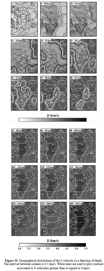
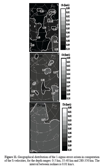
Shear velocity mapping. The above-described S-velocity distributions with depth, obtained for each grid point (or rectangular block) of the above-mentioned grid defined in the study area, are plotted with contour maps. This 3D S-velocity structure is mapped with contours by depth intervals, obtaining 2-D images of shear velocity for the study area, as shown in Figure 10. Such 2-D images are suitable for an easy interpretation and correlation, with other geophysical and geological information available for the study area. The 1-sigma errors in the S-wave velocities are also represented in 2-D images. These errors are plotted in Figure 11, for the some depth intervals, to check the error spatial distribution of the S-wave velocities mapped in Figure 10.
6. Results and discussion
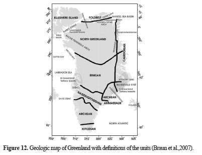
In this section, the results obtained in this study and shown in the S-velocity mapping of Figure 10, will be presented and discussed. The structural features shown by these images will be also correlated with other geophysical studies (developed in the study area) and correlated with the geology (Figure 12).
Depth range: 0 - 5 km. The S-velocity map shows clearly the distribution of sedimentary basins of the study area, located between the principal chains of mountains (Figure 8). The S-velocity presents the lowest values for the basins and the highest values for the consolidated and old structures (Figure 12). Unfortunately, the obtained results for this depth range don't can be correlated with the results obtained by other authors, because any seismic tomography (or even any S-velocity profile) never has been obtained in the depth range from 0 to 50 km, for Greenland and its surrounding area, until now. This fact is due to the absence of precise surface-wave dispersion measurements, in the period ranges from 5 to 30 s, in the previous studies (Darbyshire et al., 2004; Pilidou et al., 2005). This lack of information in these above-mentioned previous studies caused the lack of a 3D S-velocity structure (or even any S-velocity profile), for the depth range from 0 to 50 km. Thus, Figure 10 shows the first S-velocity values obtained for this study area, from 0 to 50 km of depth, and the first S-velocity mapping performed from 0 to 75 km of depth.
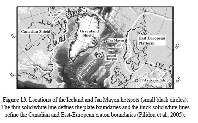
Depth range: 5 - 15 km. The geographical distribution of the S-velocity values shows an S-velocity pattern different to the S-velocity pattern obtained for the previous depth range. For this depth range, the lowest S-velocity values are not correlated with the location of the sedimentary basins. The S-velocity presents the highest values for the southern part of Greenland. Nevertheless, the S-velocity values are high in general, because Greenland's crust is mostly of Precambrian age and therefore is an old and very rigid structure, which propagates the seismic waves very well (the seismic waves travel fast and their velocities are high). The S-velocity presents the highest values for the consolidated and older structures (located mostly at the southern part of Greenland), while the S-velocity values at the north are the lowest ones for the Greenland region (Figure 12). The S-velocity shows the highest values for the Archean blocks, north and east of the Ketilidian and Nagssugtoqidian blocks, respectively. These areas of high velocity are separated by a zone of slightly lower S-velocity, associated to the Nagssugtoqidian block. The S-velocity values in the zone of the Ketilidian block also are slightly lower than those for the above-mentioned Archean blocks. The S-velocity shown for the area of the Nagssugtoqidian and Rinkian blocks, presents very similar values for both blocks, because these blocks are quite similar geologically. The S-velocity shows the lowest values of the Greenland region, in the area of the East and West Greenland Tertiary basalts, as expected for the youngest and less consolidated areas of Greenland. The S-velocity values for the area of the Ellesmere Island and the Caledonian and North Greenland Foldbelts, are similar to those shown for the northern part of the North Greenland block. It should be noted that the S-velocity shows sligthtly different values for the northern and southern parts of the North Greenland block, the S-velocities are higher for the southern part, because the southern part of North Greenland belongs to the Greenland shield, which is an older and more consolidated structure than the northern part, therefore it is a more rigid structure that propagates the seismic waves better than the northern part. In the whole study area, the lowest S-velocities are shown in the off-shore areas. For these areas, the zone of the Reykjanes and Kolbeinsey ridges shows the lowest S-velocity values, as expected for a zone of younger crust and lithosphere (Figure 13). For this low velocity zone, it should be noted that a small area of slightly lower S-velocity is just located at the Iceland hotspot, for the depth range from 10 to 15 km. For the Jan Mayen hotspot has not associated a similar low S-velocity area, probably due to an inadequate Rayleigh-wave path coverage for this area (Figure 1).
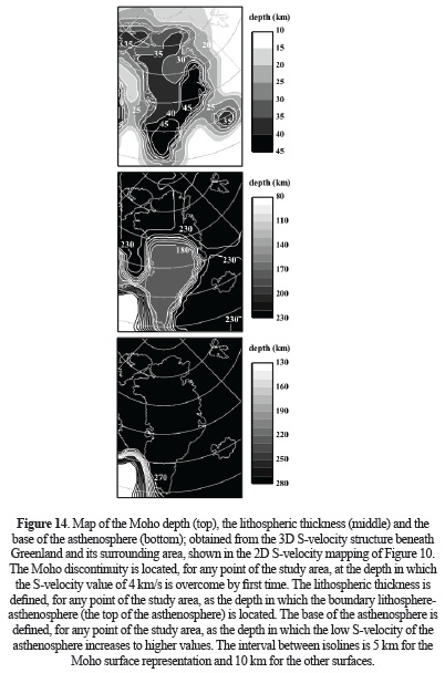
Depth range: 15 - 45 km. The geographical distribution of the S-velocity values for this depth range shows higher values (4 km/s and higher shown in Figure 10 by contours with white line) in zones of the study area in which the Moho depth is overcome (i. e. zones which the depth range considered is located below the Moho discontinuity). For each depth range shown in Figure 10 (between 15 and 45 km), the Moho depth is overcome in different areas. The Moho depth is firstly overcome in off-shore areas and lastly in on-shore and continental areas. In general, the S-velocity increases with depth for the whole study area, for each depth range between 15 and 45 km. Again, the S-velocity presents the lowest values at the north of Greenland, while the highest ones are present at the south. The S-velocity presents higher values for the consolidated and old structures (Figure 12). Nevertheless, the S-velocity difference associated to this structural difference is minor than the S-velocity difference due to the Moho depth overcoming, because the S-velocities associated with the crust are much minor than those associated with the upper mantle. Thus, if the S-velocity value of 4 km/s is used to find the Moho depth in the whole study area, considering that an S-velocity value greater than 4 km/s is associated with upper-mantle structure, then it is possible to plot a map of the Moho discontinuity, such as the map shown in Figure 14 (top), from the S-velocity mapping shown in Figure 10 (which is in fact an ensemble of 2D plots for a 3D S-velocity distribution). The Moho map shown in Figure 14 (top) agrees well with the Moho map calculated by Braun et al. (2007), for Greenland and its surrounding area. Also, a good agreement is found with the Moho depths calculated by Dahl-Jensen et al. (2003), from receiver-function analysis.
Depth range: 45 - 80 km. Again, the S-velocity presents the highest values at the south of Greenland, while the S-velocity values at the northern part are the lower. The S-velocity increases with depth for the whole study area, for each depth range between 45 and 80 km. Once again, the S-velocity presents higher values for the consolidated and old structures, which allows the identification, in terms of S-velocity, of the principal units that compose Greenland (Figure 12) . The S-velocity shows the highest values for the Archean blocks, north and east of the Ketilidian and Nagssugtoqidian blocks, respectively. These areas of high velocity are separated by a zone of slightly lower S-velocity, associated to the Nagssugtoqidian and Ketilidian blocks. Again, the S-velocity shown for the area of the Nagssugtoqidian and Rinkian blocks, presents very similar values for both blocks, as in the previous depth ranges. However, the S-velocity doesn't show low values, in the area of the East and West Greenland Tertiary basalts, opposite to the previous depth ranges. Also again, the S-velocity values for the area of the Ellesmere Island and the Caledonian and North Greenland Foldbelts, are similar to those shown for the northern part of the North Greenland block, as in the previous depth ranges. It should be noted that the difference in S-velocity values for the northern and southern parts of the North Greenland block, shown for the previous depth ranges, is very small for this depth range. In the whole study area, the lowest S-velocities are shown in the off-shore areas. For these areas, the zone of the Reykjanes and Kolbeinsey ridges (Figure 13) shows the lowest S-velocity values, as in the previous depth ranges. It should be noted that a small area of slightly low S-velocity, just located at the Iceland hotspot (Figure 13) , is also shown for this depth range. This pattern of low velocities is typical for young oceans (Evans and Sacks, 1979; Sigmundsson, 1991). On the other hand, the S-velocity values calculated in the present study agree well with those obtained by Darbyshire et al. (2004) and Pilidou et al. (2005). Nevertheless, this comparison only can be approximately done, because Darbyshire et al. (2004) didn't perform any S-velocity mapping, they only performed some S-wave velocity profiles. Respect to the S-velocity mapping performed by Pilidou et al. (2005) for the North Atlantic area (in which the region of Greenland is included), it should be noted that Greenland is a very small region, comparing with the big size of the North Atlantic area. As a consequence of this, a very poor resolution is achieved by their S-velocity mapping for Greenland and its surrounding area. Logically, the information about the Greenland structure, which can be discerned from global mappings as the mapping performed by Pilidou et al. (2005), will have always a poorer resolution than that obtained from the present study.
Depth range: 80 - 130 km. The S-velocity pattern shown for the whole study area is very similar to that shown for the previous depth range, except for the study area at the south of the Davis Strait, in which the S-velocity shows lower values respect to those in the previous depth range, because the asthenosphere is reached at this depth range and for this area, as shown in Figure 14 (middle). The lithosphere-asthenosphere boundary (or equivalently the lithosphere thickness) shown in Figure 14 (middle), has been computed from the 3D S-velocity structure, calculated in the present study and represented by the 2D S-velocity mapping shown in Figure 10, considering for each point of the study area the depth in which the S-velocity starts to decrease with depth. The map of the lithosphere-asthenosphere boundary (LAB), shown in Figure 14 (middle), is a very interesting feature obtained in the present study, which agrees well with that calculated by Kumar et al. (2005), from receiver function analysis. The LAB shown in Figure 14 (middle) is more detailed than that calculated by Kumar et al. (2005), covering Greenland and its surrounding area more efficiently. Also, it should be noted that the lithosphere thickness, for areas in which are present consolidated and old structures, shows values very similar to those calculated for areas with consolidated and old structures in other continents as South America (Corchete, 2012), Antarctica (Corchete, 2013a) or Africa (Corchete, 2013b). On the other hand, the S-velocity values calculated in this study agree well with those obtained by Darbyshire et al. (2004) and Pilidou et al. (2005), also for the present depth range. The S-velocity mapping performed by Pilidou et al. (2005) shows similar S-velocity pattern for Greenland and its surrounding areas. Nevertheless, the identification of the principal units that compose Greenland, in terms of S-velocity, is clearer in the S-velocity maps of the present study than in those performed by Pilidou et al. (2005), due to the poorer resolution achieved by their global mapping for a small area as Greenland.
Depth range: 130 - 180 km. The S-velocity pattern shown for the whole study area is very similar to that shown for the previous depth range, except for the study area at the south of the Davis Strait, because the asthenosphere is overcome, at this depth range and for this area, as shown in Figure 14 (bottom). The boundary of the asthenosphere base (or equivalently the lithosphere-asthenosphere system thickness) shown in Figure 14 (bottom), has been computed from the 3D S-velocity structure, calculated in the present study and represented by the 2D S-velocity mapping shown in Figure 10, considering for each point of the study area the depth in which the S-velocity starts to increase with depth below the LAB. It should be noted that the map of the asthenosphere base shown in Figure 14 (bottom), is a new and very interesting feature never obtained before the present study. On the other hand, the S-velocity mapping performed by Pilidou et al. (2005) shows an S-velocity pattern similar to that obtained in this study, at this depth range. Nevertheless, the poorer resolution achieved for their global mapping, in the Greenland region, makes difficult the precise comparison with the present study.
Depth range: 180 - 230 km. The S-velocity pattern shown for the whole study area is very similar to that shown for the previous depth range, except for the southern part of Greenland (in the area of the Archean, Ketilidian, Nagssugtoqidian and Rinkian blocks), in which the S-velocity shows lower values respect to those in the previous depth range, because the asthenosphere is reached at this depth range and for this area, as shown in Figure 14 (middle). This feature is also observed in the S-velocity mapping of Pilidou et al. (2005), although the poor resolution of this global mapping for Greenland makes difficult the precise comparison with the present study. The improvement in resolution achieved in this study at the deeper depths, is also related to the wide period range in which the Rayleigh-wave group velocities has been measured. In the present study, dispersion curves (group velocities) until 200 s of period have been determined, providing observed data to fit the deep S-velocity structure with more accuracy than any previous study.
Depth range: 230 - 280 km. The S-velocity pattern shown is similar to that in the previous depth range, except for the north and eastern part of Greenland (in the area of the Ellesmere Island and the Caledonian, North Greenland Foldbelt and North Greenland blocks) and for the major part of the off-shore areas which are surrounding Greenland (in the North Atlantic area of the Reykjanes and Kolbeinsey ridges, in the area of the Wandel and Labrador Seas and in the off-shore area of North Greenland and the Ellesmere Island), in which the S-velocity shows lower values, because the asthenosphere is reached, at this depth range and for this area, as shown in Figure 14 (middle). Thus, the asthenosphere is reached beneath the whole Greenland and the major part of the study area, at this depth range. For this reason, the S-velocity presents the lowest values shown for the upper mantle, as a consequence of the asthenosphere presence in the major part of the study area, at this depth range, as shown in Figure 14 (middle). Once again, this feature is also observed in the S-velocity mapping of Pilidou et al. (2005), although the poor resolution of their global mapping for this study area and this depth range (their resolution decreases drastically with depth from 200 km), makes difficult the precise comparison with the results achieved in the present study.
Depth range: 280 - 350 km. The S-velocity values shown for this depth range jump respect to those shown in the previous depth range, from low values (4.3 - 4.5 km/s) to high values (4.8 - 5.0 km/s). Obviously, the low-velocity channel associated to the asthenosphere, shown in the previous depth range, has been overcome for the whole study area in the present depth range. Also for this depth range, the S-velocity presents the highest values at the south of Greenland, while the S-velocity values are lower at the north of Greenland. The lowest S-velocity values are shown for the off-shore areas that surround Greenland. The identification, in terms of S-velocity, of the principal units that compose Greenland is more difficult for this deeper depth range, because the S-velocity differences are very small for this depth range. The S-velocity contrast decreases with depth, while the S-velocity values increase with depth. The result is an S-velocity pattern of similar high S-velocity values, for the whole study area in this depth range.
7. Conclusions
The results presented in this paper show that the techniques used here are a powerful tool for investigating the elastic structure of Earth, through the dispersion analysis, regionalization and inversion to obtain shear-velocity maps for several depths. This methodology is a good tool to investigate the physical properties of the earth structure, in any region of Earth with a variety of tectonic features, as in the present study. By means of this analysis, the principal structural features beneath Greenland and its surrounding area have been revealed. Such features include the existence of lateral and vertical heterogeneity in the whole study area, as concluded from Figure 10. The zones with consolidated and old structures present higher S-velocity values than the other zones, although this difference can be negligible in some cases. Nevertheless, the identification, in terms of S-velocity, of the principal units that compose Greenland (Figure 12) has been possible for many depth ranges. On the other hand, in the depth range of 15 to 45 km, the different Moho depths present in the study area generate the principal variation of S-velocity, because the S-velocities associated to the crust are lower than those associated to the upper mantle. A similar behaviour is found for the LAB, which generates the principal variations of S-velocities in the depth range from 80 to 230 km, because the S-velocities associated to the lithosphere are higher than those associated to the asthenosphere, as is well known. Finally, a new and interesting feature obtained in this study is the definition of the base of the asthenosphere (for the whole study area), for depths ranging from 130 to 280 km, respectively.
Acknowledgements.
The author is grateful to the National Geophysical Data Center (NGDC), the Incorporated Research Institutions for Seismology (IRIS) and the GLISN group, for providing data used in this study. The elevation data has been retrieved from NGDC, through the database: ETOPO1. The seismograms and the instrumental response have been retrieved from IRIS (through the internet utility WILBER II) and from the database: IRIS DMC MetaData Aggregator, respectively.
References
Aki K. and Richards P. G., 1980. Quantitative Seismology. Theory and methods. W. H. Freeman and Company, San Francisco. [ Links ]
Braun A., Kim H. R, Csatho B. and von Frese R. R. B., 2007. Gravity-inferred crustal thickness of Greenland. Earth and Planetary Science Letters, 262, 138-158. [ Links ]
Cara M., 1973. Filtering dispersed wavetrains. Geophys. J. R. astr. Soc., 33, 65-80. [ Links ]
Corchete V., Chourak M. and Hussein H. M., 2007. Shear wave velocity structure of the Sinai Peninsula from Rayleigh wave analysis. Surveys in Geophysics, 28, 299-324. [ Links ]
Corchete V. and Chourak M., 2010. Shear-wave velocity structure of the western part of the Mediterranean Sea from Rayleigh-wave analysis. International Journal of Earth Sciences, 99, 955-972. [ Links ]
Corchete V., 2012. Shear-wave velocity structure of South America from Rayleigh-wave analysis. Terra Nova, 24, 87-104. [ Links ]
Corchete V., 2013a. Shear-wave velocity structure of Antarctica from Rayleigh-wave analysis. Tectonophysics, 583, 1-15. [ Links ]
Corchete V., 2013b. Shear-wave velocity structure of Africa from Rayleigh-wave analysis. Int. J. Earth Sci., 102, 857-873. [ Links ]
Dahl-Jensen T., Larsen T. B., Darbyshire F. A., Woelbern I., Bach T., Hanka W., Kind R., Gregersen S., Mosegaard K., Voss P. and Gudmundsson O., 2003. Depth to Moho in Greenland: receiver-function analysis suggests two Proterozoic blocks in Greenland. Earth and Planetary Science Letters, 205, 379-393. [ Links ]
Darbyshire F. A., Larsen T. B., Mosegaard K., Dahl-Jensen T., Gudmundsson O., Bach T., Gregersen S., Pedersen H. A. and Hanka W., 2004. A first detailed look at the Greenland lithosphere and upper mantle, using Rayleigh wave tomography. Geophys. J. Int., 158, 267-286. [ Links ]
Dziewonski A., Bloch S. and Landisman M., 1969. A technique for the analysis of transient seismic signals. Bulletin of the Seismological Society of America, 59, 427-444. [ Links ]
Dziewonski A. M. and Anderson D. L., 1981. Preliminary reference earth model. Phys. Earth Planet. Inter., 25, 297-356. [ Links ]
Evans J. R. and Sacks I. S., 1979. Deep structure of the Iceland plateau. J. Geophys. Res., 84, 6859-6866. [ Links ]
Gregersen S., 1970. Surface wave dispersion and crust structure in Greenland. Geophys. J. R. astr. Soc., 22, 29-39. [ Links ]
Gregersen S., 1970. Seismicity and observations of Lg wave attenuation in Greenland. Tectonophysics, 89, 77-93. [ Links ]
Keilis-Borok V. I., 1989. Seismic surface waves in a laterally inhomogeneus Earth. Kluwer Academic Publishers, London, UK. [ Links ]
Kumar P., Kind R., Hanka W., Wylegalla K., Reigber Ch., Yuan X., Woelbern I., Schwintzer P., Fleming K., Dahl-Jensen T., Larsen T. B., Schwintzer J., Priestley K., Gudmundsson O. and Wolf D., 2005. The lithosphere-asthenosphere boundary in the North-West Atlantic region. Earth and Planetary Science Letters, 236, 249-257. [ Links ]
Pilidou S., Priestley K., Debayle E. and Gudmundsson O., 2005. Rayleigh wave tomography in the North Atlantic: high resolution images of the Iceland, Azores and Eifel mantle plumes. Lithos, 79, 453-474. [ Links ]
Sigmundsson F., 1991. Post-glacial rebound and asthenosphere viscosity in Iceland. Geophys. Res. Lett., 18, 1131-1134. [ Links ]

