1. Introduction

Soil temperature prediction is important for various agricultural purposes, especially in arid and semi-arid regions, such as Iran. Temporal patterns of soil temperatures in these regions show large seasonal and daily fluctuations. These variations in soil temperature affect plant growth directly through their effect on physiological activities and indirectly through the effect on soil nutrient availability (Tuntiwaranurk et al., 2006). For example, root growth and biological soil activity are directly influenced by soil temperature (Kang et al., 2000). Soil temperature fluctuations affect various processes within the soil such as microbial decomposition, p and k absorption, soil-moisture content (^{Elshorbagy and Parasuraman, 2008}) and soil respiration (^{Gaumont-Guay et al., 2006}).

The success of seeding efforts depends greatly on the spatial and temporal distribution of soil temperature. Thus, the temperature predictions help to improve the understanding of the dynamics of vegetation (Kang et al., 2000). It also helps agronomists and engineers to decide the proper plantation date, design drainage and irrigation systems, and to optimize the application of pesticides and fertilizers to reduce chemical pollution of soils and groundwater. For these reasons, understanding of the variation in soil temperature is vital. However there are very few climatologic stations in arid and semi-arid regions where soil temperatures are recorded at various depths. It is usually quite difficult to measure temperature at depth. To aid in this measurement process, application of data-driven models are used to estimate daily soil temperatures in ungaged homogeneous regions.

Temperatures in soil are influenced by a number of factors, such as meteorological conditions (i.e. solar radiation and air temperature), site topography, soil water content, and whether the surface is covered by litter and canopies of plants. Many conceptual models have been proposed to model soil temperature based upon the meteorological parameters such as surface global radiation and air temperature (Kang et al., 2000; ^{Shannon et al., 2000}; ^{Timlin et al., 2002}), soil physical parameters, such as water content and texture, topographical variables such as elevation, slope and aspect (Kang et al., 2000), and other surface characteristics such as leaf area index (LAI) and ground litter stores. Other models such as multiple regression and Fourier analysis have also been suggested with some modification. Most of these models are based on several assumptions and boundary conditions resulting in the limitations of their use in practice. For instance, Kang et al. (2000) developed a hybrid soil temperature model based on heat transfer physics and a relationship between air and soil temperature to predict daily spatial patterns of soil temperature in a forested landscape. They incorporated the effects of topography, canopy and ground litter.

Despite of the availability of different models to predict the soil temperature, these models are found to work well only for specific climatic and agronomic conditions under which they were originally developed. Over past decades, remote sensing techniques have also been utilized to measure and predict soil temperature over large areas but a major drawback of this approach is the availability of soil temperature data in the top few centimeters (^{Elshorbagy and Parasuraman, 2008}). The temperature of the soil profile with increasing depth is difficult to predict so that the abovementioned techniques are limited to shallow soils (^{Tyronese et al., 2008}).

Within the last decade, artificial intelligent (AI) systems such as fuzzy logic (FL) and artificial neural networks (ANNs) have effectively been used to model nonlinear and non-stationary process (^{Shiri and Kisi, 2011}). ANNs are mathematical models consisting of a network of computation nodes called neurons with established connections between them. Fuzzy logic is an alternative technique capable of generating models that incorporate expert knowledge and available measurements for a system by using a set of easily comprehensible rules in the form of a fuzzy inference system (FIS) (^{Zadeh, 1965}). A FIS is a nonlinear mapping of a given input vector to an output using fuzzy logic based on a set of membership functions and rules. Improved performance can be obtained by integrating fuzzy systems and the ANN approach to deal with large and imprecisely defined complex systems.

An adaptive neuro-fuzzy inference system (ANFIS) is one of the most successful schemes which combine the benefits of these two powerful paradigms into a single model. The goal of the ANFIS is to find a model or mapping that will correctly associate the inputs with the output.

Data mining refers to the process of searching for and discovering various patterns in data and of summarizing a set of known values to obtain the most important information (^{Quinlan, 1992}). Tree-based methods are one data mining technique and their output is a model having the structure of a tree with input and output data. The M5 model tree was introduced by Quinlan in 1992 and is a subset of data mining methods. The M5 algorithm is the most common classification used in the family of decision-making tree models. A decision tree model is essentially a decision-making tree in which linear regression equations at the leaves replace terminal class values. Within the last decade, several studies reported the use of data mining techniques such as the M5 tree model for water resource issues applications (^{Solomantine and Dulal, 2003}; ^{Bhattacharya and Solomatine, 2005}; ^{Stravs and Brilly, 2007}; ^{Pal et al., 2012}; ^{Sattari et al., 2013a}; Sattari et al., 2013b; Sattari, et al., 2014; Esmailzadeh and Sattari, 2015; ^{Biabani et al., 2016}; ^{Shortridge et al., 2016}; ^{Adnan et al., 2017}; ^{Sayagavi et al., 2016}; ^{Schnier, 2016}). However to the best knowledge of the authors, there has not been an application of the M5 tree model to predict soil temperatures at various soil depths, especially in arid and semi-arid climates. Our primary motivation in this study is to simulate soil temperatures at various depths. In this manner, it is possible to predict future soil temperatures by simply acquiring the climatic data from the meteorological stations. This is particularly important when planning future agriculture practices.

This study will evaluate the performance of various data mining techniques such as ANFIS, ANNs and the M5 tree model for estimating daily soil temperature at different depths in semi arid regions such as Iran.

2. Materials and methods

2.1 Study area and data used

Located in the central arid region of the country, the Isfahan province of Iran lies between 30o 42' to 34o 30'N and 49o 36' to 55o E (Figure 1). The altitude in this area varies from 707 to 4000 m. The significant change in altitude and its effect on climate provide various habitats and diverse plant species.

Figure 1 Location of the study area 

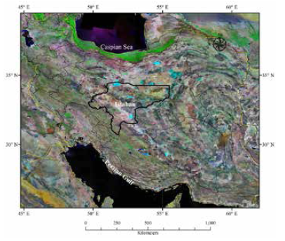
The experimentally obtained daily soil temperature and other meteorological parameters were measured at the weather station of Isfahan from 1992 to 2005. The soil temperature data were obtained for soil profiles at various depths (i.e. 5, 10, 20, 30, 50 and 100 cm). Meteorological parameters including: daily mean, minimum and maximum air temperature (Ave T, Min T, Max T), evaporation (EV), daily sunshine hours (SunH) and radiation (Ra) were also considered as inputs.

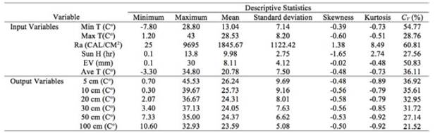
The descriptive statistics Min, Max, Mean, standard deviation, coefficient of skewness (Cs), coefficient of kurtosis (Ck) and coefficient of variation (CV) of the soil temperature and meteorological data time series, are provided in Table 1.

Table 1 Descriptive statistics of the soil temperature data 

The available data were split into two parts. The first part consists of3028 samples between June 1992 and October 2004 and was used to train different models. The second part, consisting of 335 samples between October 2004 and December 2005 was used for testing. The coefficient of determination (R2) and root mean square error (RMSE) statistics were used to compare the performance of various modeling approaches used in this study.

It is often useful to scale the input and output parameters before using them with ANNs. In the present work, input and output data were scaled to a range from -1 to +1, which is preferable when tan-sigmoid activation functions are used with the neural network. The following normalization equation was used

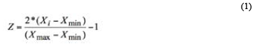
where Z is standardized input values lying in the range of [-1, + 1], and Xmin and Xmax are minimum and maximum input values, respectively.

2.2 Adaptive Neuro-Fuzzy Inference System (ANFIS)

Fuzzy logic represents knowledge using IF-THEN rules in the form of "if X and Y then Z" (^{Zadeh, 1965}). FIS mainly consists of fuzzy rules and membership functions and fuzzification and de-fuzzification operations (^{Jang, 1993}). Figure 2 shows a typical architecture of an ANFIS. In this figure, circles represents fixed nodes, whereas squares indicate adaptive nodes. The input and output nodes represent the meteorological parameters and soil temperature, respectively. The nodes in the hidden layers act as membership functions (MFs) and rules. For simplicity, it is assumed that the examined FIS has two inputs and one output. For a first-order Sugeno fuzzy model, a typical rule set with two fuzzy ''if-then'' rules can be expressed as follows:

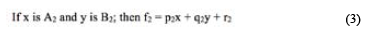
where x and y are two crisp inputs, and Ai and Bi are the linguistic labels associated with the node function. The ANFIS has the multiple layers, as displayed in Figure 2.

Figure 2 Architecture of the ANFIS 

Layer 1: All the nodes in this layer are adaptive nodes which mean that the outputs of the nodes depend on the parameters pertaining to these nodes. Each node corresponds to a linguistic label which has a membership function that may be Gaussian or any other MF.

Layer 2: Every node in this layer is a fixed node labeled as II, representing the firing strength of each rule.

Layer 3: Every node in this layer is a fixed node labeled as N, representing the normalized firing strength of each rule.

Layer 4: Every node i in this layer is an adaptive node with a node function defined as:

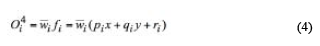
Where Oi4 is node output, wi is the normalizing firing strength from layer 3 and {pi, qi, ri} are the parameter set of this node.

Layer 5: The single node in this layer is a fixed node labeled S which computes the overall output by summing all incoming signals and is the last step of the ANFIS. The output of the system is calculated as:

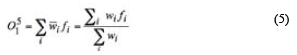
where O15( node output), is the weighted sum of right hand side polynomials in Equation 5.

The implementation of ANFIS consists of two major phases; the structure identification phase and the parameter identification phase. The ANFIS parameter estimation can be carried out by training the ANFIS system by using a hybrid learning algorithm. The hybrid learning algorithm of ANFIS consists of the two parts: (a) the learning of the premise parameters by back-propagation and (b) the learning of the consequence parameters by least-squares estimation.

In the forward pass of the hybrid learning algorithm, functional signals move forward to layer 4 to calculate each node output. The premise parameters in layer 2 remain fixed in this pass. The consequent parameters are then identified by the least-squares estimate. In the backward pass, the error rates propagate backward from the output towards the input, and the premise parameters are updated by the gradient descent (^{Shu, et al., 2008}).

2.2.1 Subtractive clustering

Subtractive clustering is an automated data-driven approach to generate primary fuzzy models. The subtractive clustering algorithm is used in case the number of clusters is not clear. This algorithm depends on the structure of the data and can be used as a dimensionality reduction tool. This algorithm can also be used to generate a fuzzy system with the minimum number of rules required to distinguish the fuzzy qualities associated with each of the clusters. Subtractive clustering is based on a measure of the density of data points in the feature space. The idea here is to find regions in the feature space with high densities of data points. Consider a collection of n data points {x1,...,xn}, subtractive clustering algorithm assumes each data point as a potential cluster center. A density measure at a data point xi is then defined as:

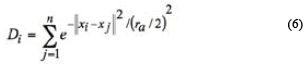
where Di is the density measure and the cluster radius rα is a positive constant (rα > 0) defining the neighborhood radius for each cluster center. Thus, a data point that has many neighboring data points will have a high potential of being a cluster center. Data points existing outside of this radius have little or no effect on the density measure.

The choice of rα is crucial in determining the cluster numbers. Large value of rα will generate a limited number of clusters, while small values of rα will generate a large number of clusters. After calculation of the potential of each vector, the one with the highest potential is selected as the first cluster center. Suppose xc1 is the point selected and Dc1 is its density measure. The density measure for each data point xi is revised by the formula:

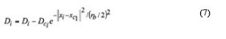
where rb is a positive constant (rb > 0) that represents the radius of the neighborhood for which considerable potential reduction will happen in density measure. In order to avoid obtaining closely spaced cluster centers, the constant rb is usually 1.5 times that of rα. Finally, the clusters' information is used to determine the initial number of rules and antecedent membership function that is used for identifying the FIS (^{Chiu, 1994}).

2.4 M5 model tree

Model trees generalize the concepts of regression trees and are analogous to piece-wise linear functions. A M5 model tree is a binary decision tree having linear regression function at the terminal nodes, which can predict continuous numerical attributes (^{Quinlan, 1992}). The M5 model tree is an algorithm for making numerical predictions, and the selected tree nodes have the attribute of maximum expected error that is a function of the standard deviation in the output parameters. A model tree based regression approach works in two different stages. In the first stage, a splitting criterion is used to create a decision tree. The splitting criterion for the M5 model tree algorithm is based on treating the standard deviation of the class values that reach a node as a measure of the error at that node and calculating the expected reduction in this error as a result of testing each attribute at that node. The formula for computing the standard deviation reduction (SDR) is:

Where

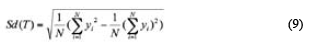
and T is a set of samples entering each node. The symbol Ti represents a subset of the samples that have the ith result of the potentiality test, Sd is the standard deviation, yi is the numerical value of the target attribute of sample i, and N the total number of data points (Alberg et al., 2012). The splitting process allows the data in child nodes to have a lower standard deviation compared to their parent node and can be considered as more pure.

After examining all the possible splits, M5 chooses the one that maximizes the expected error reduction. The division of training data with a M5 model tree produces a large tree-like structure which may cause overfitting of the data. A pruning algorithm is used to prune back the tree, for example by replacing a sub tree with a leaf in order to remove the problem of overfitting. Thus, the second stage in the design of the model tree involves pruning the overgrown tree and replacing the sub trees with linear regression functions. This technique of generating the model tree splits the parameter space into areas (subspaces) and builds in each of them a linear regression model. For further details of M5 model tree, readers are referred to related studies (^{Pal and Surinder, 2009}; ^{Quinlan, 1992}).

3. Results and discussion

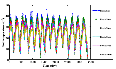
Analysis of Table 1 suggests a noticeable change in coefficient of variation (CV) value of soil temperature from the surface to the depth of 100 cm. The highest value of the coefficient of variation was observed at a 5 cm soil depth with a continuous decline in its value with increasing depth of the soil. Other statistical properties such as the maximum and mean soil temperatures are also decreasing with increasing soil depth.

It can be observed that the variability in thermal behavior of the soil profile can be a cause of this change. The higher values of coefficients of variation in the surface layers indicate that higher variability of the soil temperature at this level is possibly due to the variety of causal mechanisms influencing soil temperature. Figure 3 shows the variation of soil temperature at different soil depths in the study area. As can be seen from the figure, a wide range of fluctuations exists for the surface layers which decreases with increasing depth.

Figure 3 Time series of observed soil temperatures at different soil depths (5-100 cm) 

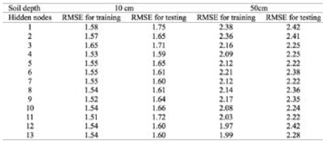
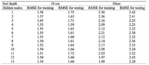
The three modeling techniques; ANFIS, ANN and M5 tree model were used to predict the soil temperature at varying depths. To obtain optimal network architecture in ANNs, the number of neurons in the hidden layer was determined by trial and error. Based on the number of input neurons (m = 6 input nodes are included here), the number of hidden nodes were varied from 1 to 2m+1 to find optimal number of nodes in hidden layer. The network was trained for 300 epochs using the Levenberg-Marquardt training algorithm. Based on a trial and error process (by exploring 1 to 2m+1 hidden neurons), hidden layers with 3, 4, 5, 4, 5 and 3 neurons were found to be optimal for the 5, 10, 20, 30, 50 and 100 cm soil depths, respectively (see Table 2 for the 10 and 50 cm soil depths).

Table 2 Tested model structures and RMSE values of the ANNs models. 

The parameters of the subtractive clustering algorithm should be specified in ANFIS models to predict soil temperatures at various depths. The clustering radius (rα) is the most important parameter in the subtractive clustering algorithm and is optimally determined through a trial-and-error procedure. The values of rα ranging between 0.2 and 1 with a step size of 0.01 were examined to minimize the root mean squared error (Table 3). For the values below 0.2, network training was found to be difficult and for the values above 1, no remarkable change in RMSE values was achieved. Clustering radius rb was selected as 1.5ra and default values of the other parameters given in the MATLAB were used.

Table 3 Resulting model structures and RMSE values of the ANFIS models. 

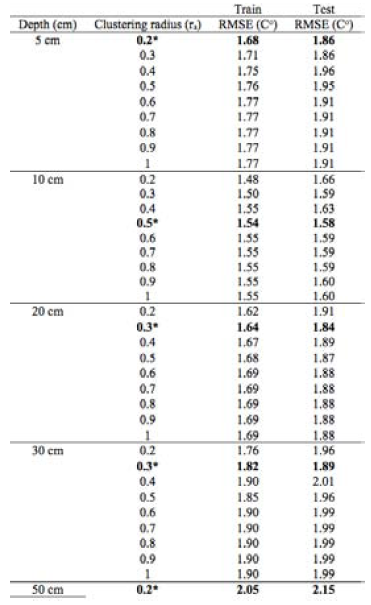
*Shows optimal Clustering radius (ra)

Gaussian membership functions were used for each fuzzy set in the fuzzy system. The number of membership functions and fuzzy rules required for a particular ANFIS model were determined through the subtractive clustering algorithm. Parameters of the Gaussian membership function were optimally determined using the hybrid learning algorithm. Each ANFIS model was trained for 100 epochs. The test results of the ANNs, ANFIS and M5 model trees are compared with respect to R2 and RMSE in Table 4.

Table 4 The test results of the optimal ANNs, ANFIS and M5 model trees. 

Results indicates a high correlation (R2 value changes from 0.98 at 5 cm depth to 0.80 at 100 cm depth) between the actual and predicted soil temperatures suggesting that all three models achieved acceptable results in predicting the soil temperatures at varying depths. Time variation and scatterplots of the test results obtained by M5 tree model, ANN and ANFIS models are illustrated in Figures 4-6.

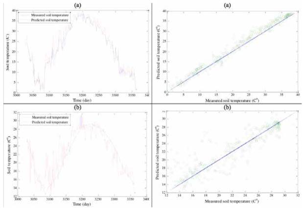
Figure 4.Plot of observed and predicted soil temperature values suggests that all three models are suitable in modeling soil temperatures. 

Figure 5 Performance of ANN model at soil depths; 5 cm and 100 cm, with test data set 

Figure 6 Performance of M5 model tree at soil depths; 5 cm and 100 cm, with test data set 

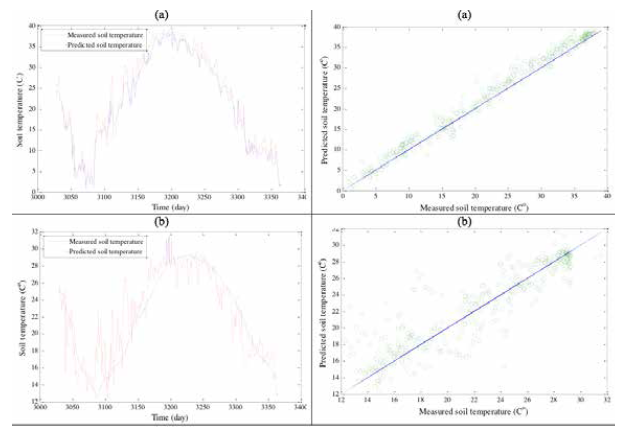
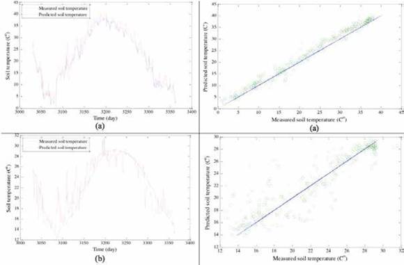
As can be seen from the Table 4, the RMSE values also increase with the increasing depth. The lowest and highest RMSE values achieved by the ANFIS, ANN and M5 tree model are 1.86, 1.95, 1.97 (observed at 5 cm soil depths) and 2.39, 2.44, 2.37 (observed at 100 cm soil depths) respectively. The plots of actual and predicted soil temperature in Figures 4, 5 and 6 as well as Table 4 suggest a slightly improved performance by ANFIS in predicting soil temperature in comparison to ANN and M5 models except at the depth of 100 cm. A comparison of results from Table 4 also suggests that both the ANN and ANFIS perform better than the M5 model tree approach in predicting the surface soil temperature, however at depth of 100 cm, M5 tree model seems to be most robust.

These figures depict good agreement between the actual and predicted soil temperature values of the surface layers in comparison to the layers at increasing depths. All three models tend to provide less biased estimates for the surface layers in comparison to the predictions for deeper layers (Figure 7).

Figure 7 RMSE values of the evaluated models for different soil depths 

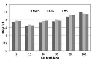
Analysis of predicted soil temperature values by different modeling approaches (Figure 7) shows increasing values of RMSE with increasing soil depth, thus indicates that the soil temperatures predicted by ANFIS, ANN and M5 models are more accurate for the surface temperatures. The reason for increasing RMSE value with increasing depth may be mainly due to the reduction in correlation between the input climatic variables and the soil temperature at increasing depth.

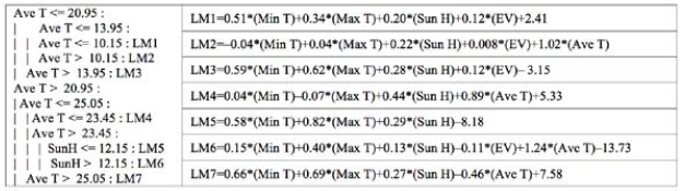
The superior performance of the ANFIS and ANN in modeling the surface soil temperatures may be attributed to the increase in the network nonlinearity and the better correlation between input and output values (^{Gao et al., 2007}). Moreover it may be noted that a trial-and-error procedure has to be adopted to select suitable user-defined parameters for the ANN model; this process is time consuming. On the other hand, no such procedure is required to develop an ANFIS model. Although error analysis of predicted values confirmed better performance for ANFIS and ANN approaches for the surface soil temperatures, the M5 model tree had slightly better results with increasing depth. It is worth noting that M5 model trees being analogous to piecewise linear functions, provides a simple linear relation to model the soil temperatures, as described mathematically in Figure 8.

Figure 8 Linear functions for predicting temperature at 5 cm soil depth based on M5 tree model. 

4. Conclusions

The ANFIS, ANNs and M5 tree model approaches have been used to predict the daily soil temperature with increasing depth in this study. The results presented here are quite encouraging and confirm that all three approaches work well in predicting soil temperatures at different depths. A comparison among the models indicates that the ANFIS model provides more accurate estimates of soil temperature than the ANNs and M5 tree model. The results also suggests that both ANN and M5 tree model approaches work well in predicting daily soil temperatures, however, M5 tree model has simple linear relations that can be easily used to predict the daily soil temperature data by field engineers. Error analysis of temperature predictions at different soil depths indicates that all three models perform well in predicting surface soil temperature data rather than at deeper depths. The reason behind this may be the fact that there is a strong relationship between climatic parameters and surface soil temperature. The results of the present study demonstrate that the proposed ANFIS model is quite efficient in predicting soil temperature for the surface layers however further investigation is needed with different data sets to compare proposed approach and other mathematical methods such as time series modeling to model soil temperatures in deeper layers.