


 English (pdf)
 Article in xml format
 Article references
 Send this article by e-mail
 Cited by SciELO
  Cited by Google
  Similars in
SciELO
Similars in
SciELO  Similars in Google
 Permalink
Introduction
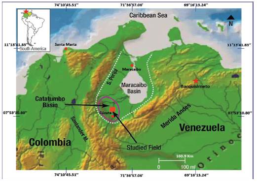
Machine learning algorithms have been broadly applied in geosciences in the latest years, most of them focus on searching natural patterns and samples classification in huge datasets. The support vector machines (SVMs) are part of supervised algorithms of machine learning methods with straightforward application and flexibility dealing with continuous and discrete data. In this opportunity SVMs have been applied to borehole logs of oil wells in the former Barco Concession, Norte de Santander Department - Colombia (Figure 1). The wells in the area were drilled in a mixed sequence, mainly of carbonates and clastic sedimentary rocks, where certain kind of limestones have been reported as hydrocarbon producer; in this research two SVMs were trained to identify automatically sections with fossiliferous limestones and intervals of calcareous shales interbedded with limestone; the remaining carbonates rocks, not classified by the SVMs, were grouped as carbonate laminated rock by applying a logic function. The objective of this model is to provide information to the well site geologist shortly after open hole logs are acquired, avoiding problems related to time consuming activities of data interpretation. The SVMs were developed with the free platform for data mining KNIME 2.7.4 (Konstanz Information Miner, 2013) using data of a pilot well (PC-7), which has detailed image logs interpretation integrated with core-logs correlation; additionally, this well has the best coverage of the target formations in the field. The SVMs generated with PC-7 data were then applied to other five well of the field (named PC - 6, PC - 8, PC - 9, PC - 10 and PC - 11). The set of logs were chosen because on one hand, nuclear logs provide information regard mineral composition and porosity of rocks; on the other hand, resistivity of imaging tool along with fractal dimension of the images provide information about textural features of logged formations (Leal, 2014). The studied section in each well were rocks of Aguardiente Formation (Uribante Group), Capacho Formation (locally called Cogollo Formation in the area of old Barco Concession), and finally the data comprise the lower part of La Luna Formation (Barrero et al., 2007).
2. Geological Setting
The Catatumbo Basin is limited by the Serrania of Perija and Santander Massif to west-southwest and Merida Andes to southeast (Figure 1). The Cretaceous rocks are limestones, shales and marine sandstones deposited in shallow sea environments that extended across northern Venezuela and continued south through Colombia to the south; Cenozoic rocks are fluvial deltaic shales and sandstones that were deposited in a foreland basin. Traps are wrench controlled and faulted anticlines resulted from strike-slip convergence. Oil was sourced mainly from the Upper Cretaceous formations La Luna and some intervals of Capacho, as well as the Lower Cretaceous Uribante Group; oil generation began in the Late Eocene and continues through today (Barrero et al., 2007). The sedimentary records of Catatumbo Basin began during syn-rift stage of Cordillera Oriental (Branquet, et al., 2002) with normal faults controlling sedimentation. The basement consists of metamorphic rock of Cambric - Silurian ages according oil wells perforated in the area (SGC, 2015). From Middle Triassic to Upper Jurassic, the Pangaea supercontinent starts its separation with an oceanic expansion zone between North America and Gondwana, both continents presenting passive margins at each side. Transform faults were produced in intra-continental zones, also producing graben structures along Colombian territory (SGC, 2015). Those grabens were filled with volcano-sedimentary rocks of La Quinta Formation, which is not cropping out in the area of old Barco Concession, but some tuffs have been recorded during perforation of wells.
A marine transgression began at Aptian times in the basin, starting sedimentation of Tibu-Mercedes formations and creation of the link between Maracaibo and Magdalena River basins (Toussaint et al., 1995). This marine transgression was produced by a slow cooling lithosphere process allowing regional thermal subsidence (SGC, 2015). The Catatumbo sequence studied in this research was deposited from Aptian to Coniaician, where succession of tectonic events along with right environmental conditions allowed sedimentation of several calcareous lithologies, resulting in a very rich petroleum system which have been producing hydrocarbon since the beginning of the last century.
2.1 Aguardiente Formation
The Aguardiente Formation of Lower Cretaceous age was partially drilled in the six studied wells of the field (Figure 2). In the area, this formation is composed of calcareous from fine to coarse-grained cross-bedded glauconitic sandstone (Notestein et al., 1944); in very low proportion beds and thin laminated carbonaceous-micaceous shales and thin beds of laminated limestones can be observed (ECOPETROL, 2012). Calcareous sandstones of this formation appear with light colors in resistive image (low conductivity), also shows low gamma rays reading and density mainly dominated by sandstone matrix. Abundant glauconite and local concentrations of shell fragments indicate deposition in a marginal marine environment, where sediments rework was conducted by tidal or wave action. It is considered that this sequence may have been deposited in marginal marine environments representing an estuarine sedimentation in this part of the basin (AIP, 2009).
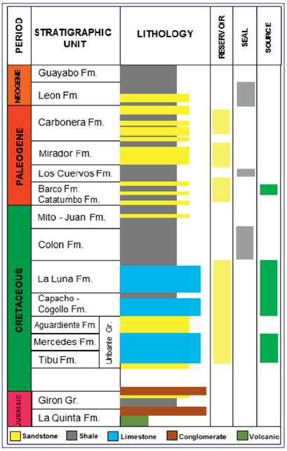
2.2 Capacho Formation
The Capacho Formation (Upper Cretaceous - Figure 2) is mainly composed of dark-gray to black shales, interbedded with fossiliferous limestones, laminated limestone and much less proportion fine-grained arenites and siltstones (ECOPETROL, 2012). The upper section consists of limestone with bivalves (oysters - fossiliferous limestones), while the rest of the section presents calcareous shales interbedded with limestone containing varying amounts of planktonic foraminifera, glauconite, calcium phosphate and organic matter. Fossiliferous limestones appear with light color and high resistivity sections in borehole images; shales show high gamma rays reading with density matrix mainly related to clay minerals. Total organic carbon reported for this formation is 2.1 % with hydrogen index of 350 mg HC/g and it is considered one of the source rocks in the basin (Gonzales, et al., 2009). The rocks of lower part in this Formation were deposited in less oxygenated deep marine zones, while rocks found in the top are associated with shallow marine deposits (AIP, 2009). The Capacho Formation was totally drilled in the six study wells showing thickness from 253.59 m to 282.24 m.
2.3 La Luna Formation
The Upper Cretaceous La Luna Formation (Figure 2) was partially logged in the wells of this research and it mainly consists of calcareous shale interbedded with limestone. The lithologies in this formation are composed of hard dark-gray abundantly foraminiferal limestones and hard black highly calcareous platy bituminous shales. Bands and nodules of black chert are present in very minor amount, more numerous in the upper part. Concretionary masses of dense gray limestone, ranging from few centimeters to 75 centimeters in size, are characteristic of the formation (Notestein et al., 1944). This formation shows high/medium gamma rays reading with density matrix and photoelectric factor related to carbonate minerals. Total organic carbon for this formation is 3.20 % with hydrogen index of 300 mg HC/g (Gonzales, et al., 2009), and it is considered the main source rocks for the entire basin in Colombia and Venezuela (Maracaibo Basin). The textural features interpreted are indicating deposition in normal marine conditions, clearly offshore, but not in open marine environments (AIP, 2009). There have been reported hydrocarbon production from naturally fractured intervals in La Luna Formation (Notestein, et al., 1944), probably related to calcareous shale interbedded with limestone sections similar than observed in the six wells of this research.
3. Data Sets
3.1 Gamma Ray Logs
Gamma ray logging is a kind of nuclear measure of natural radioactivity in formations and can be used to identify lithologies, correlating zones and determination shale (clay) volumes (Track 2 - Figure 3). Shale-free sandstones and carbonates have low concentrations of radioactive material and present low gamma ray readings. As shale content increases, the gamma ray response increases because of the concentration of radioactive material in shale. However, clean sandstone (i.e., with low shale content) might also produce a high gamma ray response if the sandstone contains radioactive minerals, or uranium-rich waters (Asquith G. & Krygowski, D., 2004). The gamma ray data in this research correspond to the total count of radioactive elements in the formation, without differentiating the Th, U, K and other radioactive minerals content.
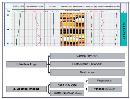
3.2 Photoelectric Factor
The photoelectric factor is a continuous record of the effective photoelectric absorption cross section index or "Pe" of a formation. The photoelectric absorption index is strongly dependent on the average atomic number, "Z", (i.e. atomic complexity) of the constituents of the formation, which implies the composition and by inference, the lithology. In the correct borehole environment, it can be used as quantitative indicator of lithology and certain diagenetic minerals. The use of this log is severely restricted by the fact that it is ineffective in holes with barite weighted mud, since the photoelectric absorption index for barite is nearly 150 times than most of the common minerals and when present will dominate the log response (Rider, 2000); the logs of the wells in this research were acquired in free barite muds (Track 3 - Figure 3).
3.3 Neutron Logs
Neutron logging (Track 4 - Figure 3) is expressed in porosity units and it is based on nuclear principles that measure the hydrogen concentration in the empty space of the rocks. In clean formation (i.e., shale-free) where the porosity is filled with water or oil, the neutron log measures liquid-filled porosity. Neutrons are created from a chemical source in the logging tool; when these neutrons collide with the nuclei of the formation they lose some of its energy. With enough collisions, the neutron is absorbed by a nucleus and a gamma ray is emitted. Because the hydrogen atom is almost equal in mass to the neutron, maximum energy loss occurs when the neutron collide with a hydrogen atom. Therefore, the energy loss is dominated by the formation hydrogen concentration (Asquith G. & Krygowski, D., 2004).
3.4 Borehole Electrical Imaging
The resistive image logs are acquired in wells without casing providing a two dimension image ofthe borehole with vertical resolution of 5.08 millimeters (Track 5 - Figure 3). Image logs allow sedimentary structures characterization, thin layers evaluation, electrofacies analysis and fractures identification. The images processing follows a standard sequence, beginning with data quality control of magnetometer and accelerometer measurements, which provide information about accurate position of all elements of the tool in space and therefore orientation of all handpicked geological features. Then, corrections of velocity and acceleration that the tool had at moment of data acquisition are performed. Finally, dynamic and static normalizations of resistivity data are applied; dynamically every foot in order to have a clear view of rock details and statically of whole logged interval optimizing tool operations under extreme resistivity. A color code is used to interpret resistive image logs, where light colors represent high resistivity and dark colors indicate low resistivity values. The most commonly observed geological events in image logs are well-defined planes which can be associated with bed boundaries, sedimentary structures, faults and fractures. These features are observed as sinusoids on image logs corresponding to the traces of planar events in the borehole.
3.5 Mean and Variance of Resistivity Pads
The mean and variance of resistivity measured by image tool are calculated after image processing and can be seeing in the tracks 6 and 7 of the Figure 3; the mean resistivity log "  " is generated from the arithmetic mean of resistivity measurements for each pads of the image tool in a specific depth, applying the equation (1).
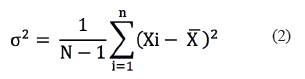
Where "" represents the average resistivity log and "n" number of resistivity measurements of each pad at a specific depth "Xi". In other hand, the variance of resistivity pads "σ2" comes from the mean resistivity log using the equation (2).
3.6 Fractal Dimension Of Borehole Image
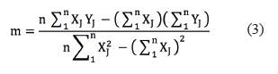
In 1975 Benoit Mandelbrot named fractal (from latin fractus -irregular), the set of forms normally generated by process of repetition characterized for having details in any observed scale (self-similarity), infinite length and fractional dimension; a dimension is fractal when the object occupies a space expressed by a fractional or decimal number (Mandelbrot, 1983). The Box counting method is widely used to find fractal dimension of diverse kind of images, where the studied figure is inserted in a box of side (r), then this box should be divided into four boxes with side "r/2" and the number of boxes covering any part of the figure "N(r)" must to be counted; following, resulted boxes are divided again into four boxes and the number of boxes "N(r)" containing any part of the figure must to be re-counted. This procedure is repeated, also counting the number of boxes with some part of the figure in order to plot the logarithm of the inverse size of boxes versus the logarithm of boxes with any part of the figure, or "|Xj"=Log (1/rJ)|" and "YJ = Log (NJ)". Finally, the slope "m" of the regression is the fractal dimension of the image obtained with the equation (3); the regression is the fractal dimension of the image obtained with the equation (3).
The Figure 4 shows example with the Sierpinski's carpet and a section of resistive image, both figure with their regression and respective fractal dimension calculated with box counting method.
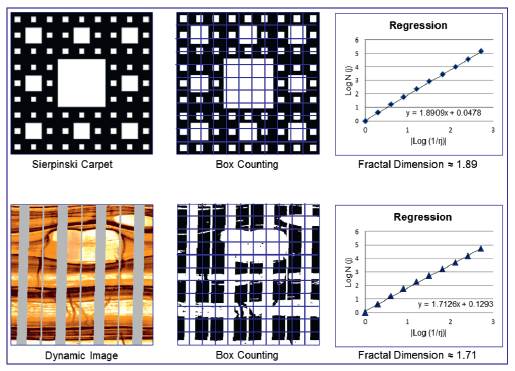
The box counting method was applied to resistive image logs with dynamic normalization in format of bit mapped picture (BMP) with 512 pixels wide by 15378 pixels long, generating a fractal dimension curve along resistive image (Track 8 - Figure 3), with sampling rate of 16.26 centimeters. The conversion of pixels to depth of images with vertical scale 1:5 is 512 pixels equal to 65.05 centimeters (Leal, et al., 2016).
4. Methods - Support Vector Machines & Logic Function Applied
A SVM is a supervised classification technique that has received considerable attention during the latest years (Tan, et al., 2006); this technique is based on statistical learning theory and has shown promising empirical results in many practical applications, including hand writing digit recognition, earthquake characterization (Ochoa, et al, 2017), and other application related to pattern recognition. The SVM also works very well with high-dimensional data and avoids the course of dimensionality problem. Another unique aspect of this approach is that it represents the decision boundary using a subset of the training example, knows as the support vectors (Tan, et al., 2006). The SVM learning problem can be formulated as a convex optimization problem, in which efficient algorithms are available to find the global minimum of the objective function. Other classification methods, such as rule-based classifier and artificial neural networks, employ a greedy-based strategy to search the hypothesis space (Tan, et al., 2006), such methods in their basic approach tend to find only locally optimum solution and are not straightforward applicable to the data set used in this research. Furthermore, SVM performs capacity control by maximizing the margin of the decision boundary. Nevertheless, the user must still provide other parameter such as the type of kernel function "K" to use and the cost function "C" for introducing each slack variable (Tan, et al., 2006). The kernel function project a dataset in a space of specific characteristics and uses algorithms related to linear algebra, geometry and statistics to identify linear patterns in the dataset. Any solution using kernel methods comprises two phases; first phase consists of a module that performs a mapping of the projected data; second phase contains an algorithm designed to detect linear patterns in the space where this data is projected (Taylor & Cristianini, 2004). The kind of kernel applied in this research was a normalized polynomial (equation 4).
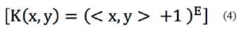
Where "E" is a parameter representing the polynomial degree and "K" represents the kernel function depending on variables "x" and "y".
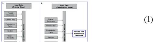
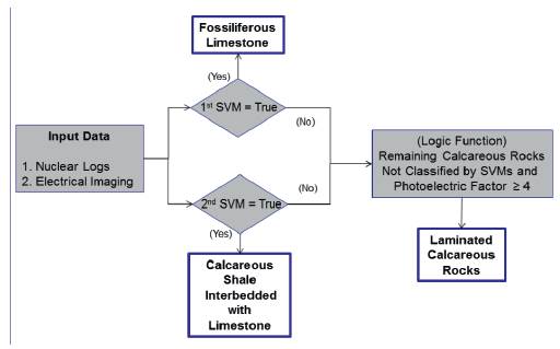
In order to identify automatically intervals with fossiliferous limestone and calcareous shale interbedded with limestone two sub-models based on SVMs were trained. During training stage the first SVM employs neutron, photoelectric factor and gamma rays logs; also in this stage is included mean and variance of resistivity measured for image tool, as well as fractal dimension of borehole image calculated with box counting. This SVM is trained with interpreted interval composed of fossiliferous limestone of the pilot well, which has core-image log calibration. During classification stage only nuclear logs, mean and variance of resistivity tool and fractal dimension of borehole image are required to find an automatic indicator of intervals with fossiliferous limestone, which are important for their hydrocarbon production in some intervals of Capacho Formation. The Figure 5 shows a sketch of this SVM in training and classification stages.
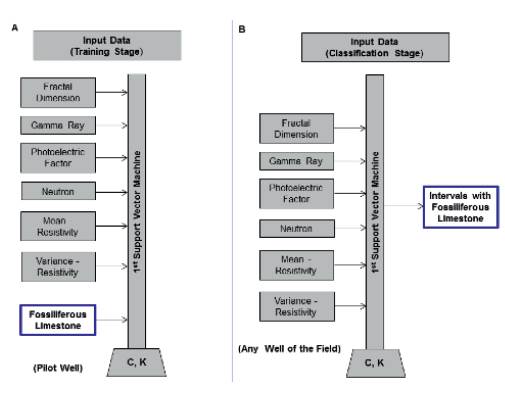
Figure 5 SVM sketch for automatic identification of fossiliferous limestones in training (A, left) and classification (B, right) stages.
In a similar way, the second SVM was trained with nuclear logs, image tool resistivity and fractal dimension of borehole images, but in this case, it was trained with interpreted intervals of calcareous shale interbedded with limestone of the pilot well (Figure 6). During classification, information of calcareous shale interbedded with limestone is not required and then this SVM automatically draws a flag where these lithologies are present, only using the data showed in the Figure 6B. The task of this SVM is important because fractured intervals of calcareous shale interbedded with limestone have been reported as hydrocarbon producer in La Luna Formation.
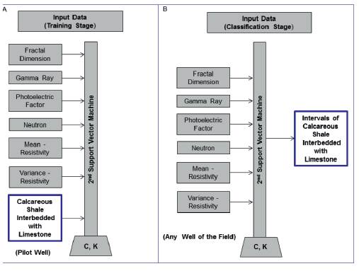
Figure 6 SVM sketch for automatic identification of calcareous shale interbedded with limestone in training (A, left) and classification (B, right) stages.
The rest of calcareous rocks present in the studied sequence are easily recognize using a logic function, where all sections with photoelectric factor equal or higher than 4 are classified as laminated calcareous rocks, as long as they were not previously classified by the first SVM nor the second. The Figure 7 shows the model applied to identify calcareous lithologies in the study area and also relationship between the logic function and SVMs.
4.1 Confusion matrices applied to evaluate the model
The performance evaluation of a classification model is based on the counts of test records correctly classified, comparing with the interpretations of a geologist. These counts are organized in a table known as a confusion matrix. In this research each classification is considered as a two-class case with classes yes and no ("there are" or "there are not"), where each single classification has four different possible outcomes shown in the confusion matrix for a binary classification of Table 1.
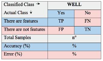
The true positives (TP) and true negatives (TN) are correct classifications. A false positive (FP) occurs when the outcome is incorrectly classified as yes (or positive) when it is actually no (negative). A false negative (FN) occurs when the outcome is incorrectly classified as negative when it is actually positive. The true positive rate is TP divided by the total number of positives, which is TP plus FN; the false positive rate is FP divided by the total number of negatives, (FP plus TN). The overall accuracy percentage is the number of correct classification divided by the total number of classification multiplied by 100% (equation 5), being the error 100 % minus this.

In order to evaluate the logic function and SVMs performance, confusion matrices were applied to the five analyzed wells. It is important to notice that data in bad hole condition was removed because of logging tools are affected along these intervals and their measures do not reflex real properties of the rocks. The sampling in confusion matrices was taken each 16.26 centimeters; therefore 1000 samples represent around 162.6 meters of length in the wells. The sampling rate of fractal dimension curves is also 16.26 centimeters (from the box counting processing), as well as it is the interpolated sampling rates of nuclear and resistivity logs data.
5. Results and Discussion
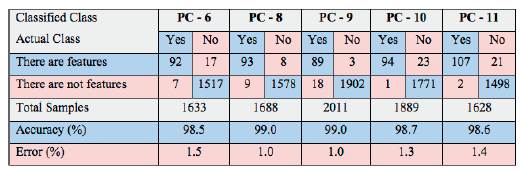
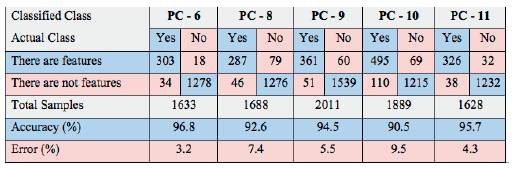
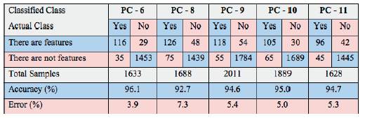
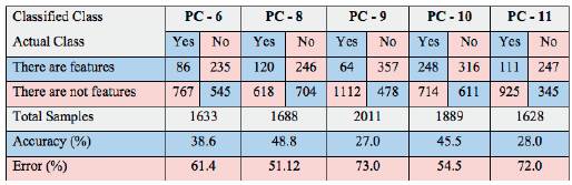
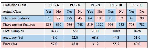
According confusion matrix, the first SVM applied to identify fossiliferous limestones presents an average accuracy of 98.8%, with best classification in the wells PC-8 and PC-9, counting 1671 samples correctly of 1688 (PC-8) and 1991 correct samples of 2011 for the well PC-9; the lower performance for this SVM was in the well PC-6 with 98.5%, where 24 samples were wrongly classified of 1633, as shown in confusion matrices of Table 2. In other hand, identification of interval with calcareous shale interbedded with limestone was performed by the second SVM, having average accuracy of 94.0% and best execution in the well PC-6 with 96.8%, counting 1581 samples correctly of 1633; lower performance was in the well PC-10 with 90.5% where 179 samples were wrongly classified of 1889, as shown in Table 3. Finally, the logic function used to identify laminated calcareous rocks, has average accuracy of 94.6%, with best performance in the well PC-6 with 96.1%, counting 1569 samples correctly of 1633 and lower execution in the well PC-8 with 92.7%, where 123 samples were wrongly classified of 1688 (Table 4).
The final representation in a common log template is shown in track 3 of Figure 8; the gamma rays and resistivity image are in track, 2 and 4 respectively. The Figure 8A shows an interval composed of calcareous shale interbedded with limestone in La Luna Formation. The Figure 8B shows example of fossiliferous limestone and laminated calcareous rocks.
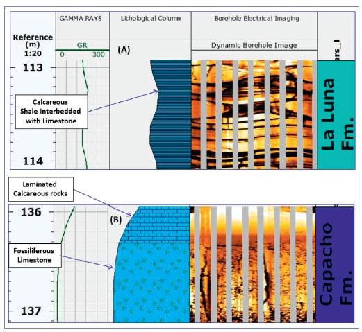
Figure 8 Track 3 shows the model representation in a typical log template, calcareous shale interbedded with limestone flag is presented in a section of La Luna Formation and a contact between laminated calcareous rock and fossiliferous limestone is presented in Capacho Formation
5.1. Fractal dimension impact on modeling performance
In order to test the impact of the fractal dimension in the identification of calcareous lithologies, the same process was executed but omitting the fractal dimension curve. This test verifies the importance of the fractal dimension and the value of its generation using box counting method.
The Tables 5 and 6 show the model performance classifying intervals of fossiliferous limestone and calcareous shale interbedded with limestone respectively. The average error increase from 1.24% to 38.88% for the 1* SVM and from 5.98% to 62.42 % for the 2nd SVM. The Table 7 shows the confusion matrix for classification of laminated calcareous rock, applying the logic function to remaining sections not classified for the SVMs and photoelectric factor > 4, in this case the error increased from 5.38% to 48.17%.
Table 5 Confusion matrix - Intervals of fossiliferous limestone - 1st SVM without fractal dimension.
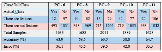
Table 6 Confusion matrix - Intervals of calcareous shale interbedded with limestone - 2nd SVM without fractal dimension.
6. Conclusions & Recommendations
The average accuracy of the model was 95.8% in five evaluated wells and it can be applied to recognize calcareous lithologies in this part of the basin, where the sequence is composed of mixture between clastic and carbonate; also their accuracy is higher enough to be automatically implemented during identification of intervals with capability to produce and storage hydrocarbon in the field, as in the case of fossiliferous limestones and calcareous shale interbedded with limestone, if this last is affected by natural fractures.
The fractal dimension of resistive image logs along with nuclear and resistivity borehole measures can be applied to identify textural features of the formation. The average accuracy decreased from 95.8% to 50.2% when the whole model was execute without the fractal dimension curve, highlighting the contribution of this approach in textural rocks classification using borehole logs.
This methodology can be applied to the rest of the wells that has the same dataset in the field, improving the sedimentological knowledge in areas without core information. For research projects in the future, the SVMs can be trained to identify sedimentary structures in borehole image of clastic rock, common in Aguardiente and middle part of Capacho formations.
SVMs are algorithms of very simple implementation; therefore, the proposed model can be applied shortly after image logs are acquired, specifically after their processing but previous their interpretation. However, the SVMs of this research must to be recalibrated in case to be applied in other field of the basin.

