Inglés (pdf)
 Articulo en XML
 Referencias del artículo
 Enviar articulo por email
 Citado por SciELO
  Citado por Google
  Similares en
SciELO
Similares en
SciELO  Similares en Google
 Permalink
Introduction
Seismic velocities play a vital role in the determination of lithology, porosity and fluid content. Seismic velocities vary horizontally and vertically depending upon the geological constraints, the depositional environment, overburden pressure, lithological variations, and others. Elastic impedance inversion is based on the assumption of using S-wave to P-wave ratio of the nth layer, and n+1 layer across the interface which is known as Κ and its value is 0.25. In this research, the effects of using Κ as constant in elastic impedance inversion have been studied. As the seismic velocities change with the variation in both the elastic properties and other geological constraints, Κ also changes accordingly.
Conventional acoustic impedance (AI) inversion, which is the product of P-wave velocity and density, assumes that the P-wave strikes the subsurface interfaces at normal incidence (Lindseth, 1979). This assumption remains valid when the offset range is small, and the reservoir is deep. However, in the presence of AVO at larger offsets the reflection coefficients and polarities may change from those at normal incidence (Ma, 2004). The elastic impedance approach provides better inversion results than the standard intercept-gradient approach which can be influenced by noise (Cambois, 2000). Elastic impedance inversion is the generalization of acoustic impedance for the variable angle of incidence.
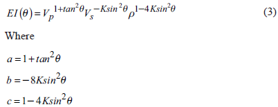
Elastic impedance inversion (EI) is the latest development in the ield of geophysics. The idea of elastic impedance was presented by Connolly (1999). He describes the importance of elastic parameters inversion to identify the fluid and lithology. Aki and Richards (2002) approximation of Zoeppritz (1919) equations and Connolly (1999) defined equation 3 (Appendix I) for elastic impedance. It is the product of P-wave, S-wave velocities, and density. Elastic impedance enables geophysicists with an additional tool for the reservoir prediction. Acoustic Impedance alone cannot distinguish and identify the fluid type and lithology. The acoustic impedance log ignores AVO effects, which enhances the chances of information loss (VerWest et al., 2000). As the P-wave velocity is a function of the mineral constituents, it can only give information regarding the geometry of pores and volume of fluid (Cosban et al., 2002). Elastic impedance uses the necessary elastic parameters of the earth such as P-wave, and S-wave velocities and density. Poisson ratio is lithologically sensitive and helps in distinguishing sandstone from mudstone, in reservoir characterization, and fluid identification.
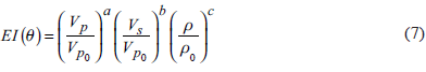
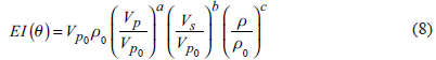
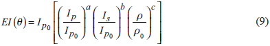
VerWest et al. (2000) presented another form of elastic impedance inversion by introducing a planar boundary between two layers of acoustic media, which depends on ray parameters. Whitcombe (2002) gave a normalized form of elastic impedance equation 7 (Appendix I). Other researchers presented different approximations of the Zoeppritz equation to provide several kinds of elastic impedance equation. Whitcombe et al. (2002) introduced the term Extended Elastic Impedance (EEI) to identify both fluid and lithology using the elastic impedance. Duffaut et al. (2000) gave the shear-elastic impedance to estimate the ratio of P-wave velocity and S-wave velocity using joint P-P and P-S elastic impedance inversion. To deal with the dimensionality problem, Savic et al. (2000) defined the elastic impedance as the function of P-wave, S-wave velocities, and ray parameters. Martins (2002)set out the elastic impedance in weak anisotropic media. Based on Fatti approximation of the Zoeppritz equation, Wang et al. (2008) proposed an elastic impedance equation by using Fatti Approximation equation 9 (Appendix I). Other elastic impedance relations are presented using different media or parameterization. In this research, the importance of the value of Κ for each AVO type has been used.
As seismic velocities increase with depth, then their effect at large offsets in depth also varies. The principal purpose of this study is to check the impact of variation in the value of Κ when used for specific data sets. Usually, Κ= 0.25 is used in elastic impedance inversion. However, due to lateral and horizontal variation in the velocity, Κ should also change accordingly, instead of using a constant value. AVO classes have been evaluated by applying the elastic impedance equations for a continuous and calculated Κ. This study will be helpful for geoscientists as well as exploration and production companies to identify the lithological reservoirs more accurately without erroneous results.
Constant K
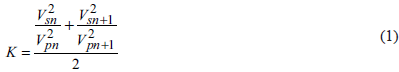
Connolly's elastic impedance equation assumes using S-P wave velocity ratio Κ as a constant for the whole data set, which is an unrealistic approach. It is the average v 2 S / V 2 p of the nth layer and n+1 layer across the interface which gives different values of Κ at the top and bottom of a layer. Hence giving different elastic impedance values.
However, for the multilayer strata, its value is taken as an average of for each layer. Mostly the rocks have V 2 S / V 2 p = 0.5, i.e., Κ = 0.25 (Connolly, 1999). It is not reasonable value as it assumes that the velocity ratio of P and S waves of each medium remains the same which is not possible because seismic velocity generally increases with depth (Ma, 2004). Lu and A. McMechan (2004) used a variable value of Κ based on empirical approximations. Elastic impedance inversion with different Κ values gives different values of Poisson's ratio estimation, which shows that it is sensitive to the choice of Κ (Mallick, 2001). Ma (2004), and Santos and Tygel (2004)introduced the term Reflection Impedance (RI), which is derived by integrating the reflectivity along the ray path to overcome the limitations of constant V 2 S / V 2 p ratio and normalization of the elastic impedance. In their study, the density is assumed to be related to the S-wave velocity(Potter et al., 1998). Most of the AVO/EI equations assume the angle of incident and value of Κ as a constant which generates errors with the increase in angle, prominently seen from the AVO/EI equations. The value of Κ should be used as a constraint rather taking as constant to minimize the errors that arise in the inversion (Jin et al., 2015). The interpretation of the results of the normalized form of the elastic impedance depends on Κ and the normalization parameters (Zhang et al., 2012).
Classification of AVO Anomalies
The intercept/gradient method is not only a good indicator of reservoirs, but this approach can also be used to classify AVO anomalies. Rutherford and Williams (1989) categorized various AVO trends as they diversified with increasing incident angle for the top of gas-saturated reservoirs. Based on field studies, they developed an AVO anomaly classification scheme for gas-saturated reservoirs. The Rutherford and Williams (1989) classification is as follows:
Class I. Gas-sand reservoir has larger impedance than the impedance of the encasing shale. Typically, normal-incident values (NI) are higher than +0.03.
Class II. Gas-sand reservoir has nearly the same impedance as the encasing shale. NI typically ranges between ±0.03.
Class III. Gas-sand reservoir has a lower impedance than the encasing shale. NI is usually less than -0.03.
Class IV. Gas-sands for which the reflection coefficients decreases with increasing offset.
Rutherford and Williams (1989) also indicated that the slope of the reflection coefficient curve is usually negative for all classes and magnitude of the gradient decreases from Class I to Class III anomalies. J.P Castagna et al. (1998) added Class IV to the Rutherford and Williams classification of AVO. They concluded that certain Class III gas-saturated anomalies have slowly decreasing amplitudes with offset and may even reverse polarity within the common depth point CDP gather. It is a reservoir with a negative AVO intercept and positive AVO gradient. Their classification demonstrates that reflection coefficients do not always have negative slopes for gas sands. However, they cautioned that the AVO gradient for Class IV brine-saturated sand might be almost identical to the AVO gradient from Class IV gas-saturated sand. Hence the gas may be difficult to detect by partial offset stacks.
Methodology
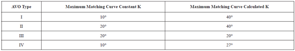
In this paper, two-layer models based on four AVO Classes which included AVO Type I, Type II, Type III, and Type IV were used. AVO type is a continuously distributed property of the seismic data (Young & LoPiccolo, 2003). The input parameters of all four models are given in Table 1. From each derived elastic impedance equation, different elastic parameters by inversion can be obtained. Connolly's elastic impedance equation and Fatti based elastic impedance equations were used for checking the behavior of value of Κ and determining which value of Κ should be utilized. Reflection Coeficient (RC) curves based on the Zoeppritz equation and Elastic Impedance equations are used for comparison of the results. MATLAB software tool is utilized to generate the plots between the reflection coefficient and offset angle. The reflection coefficient is plotted on y-axis while offset angle of 0°-40° is plotted on the x-axis.
Table 1 Parameters used for each AVO type for elastic impedance inversion, modified from Sayers and Rickett (1997)and John P. Castagna and Swan (1997)

Sayers and Rickett (1997) provided the parameters for the AVO's type I to type III, while John P. Castagna and Swan (1997) provided the type IV. The value of Κ is calculated for each AVO class using equation 1. This value varies with the change in the P-wave and S-wave velocities as shown in Table 1. These estimated values of Κ are used during generation of reflection coefficient curves for elastic impedance.
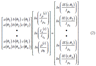
Two steps are involved in seismic inversion. First is the estimation of the subsurface reflectivity as a function of the angle of incidence for each point. Second is the inversion of reflectivity to estimate the corresponding earth parameters (Grossman, 2003). The elastic impedance allowed to calibrate far offset angle stack like acoustic impedance logs are used to calibrate zero-offset data. There are various approaches for quantitative estimation of reservoir properties from seismic inversion. In this research, the generalized matrix inversion was used. Well-X is used in the application of the findings from which the synthetic angle traces at 10°, 15°, 25° were obtained using Fatti's three-term elastic impedance formula. After generation of elastic impedance values at different angles, inversion procedure was applied; P-Impedance, S-impedance, and density of the following equation were inverted. (Equation 2 in appendix 1 will give rise to the equation.).
The 5% of random noise with Gauss distribution is added to the synthetic angle traces to test the elastic impedance inversion method. Calculated log of Κ is generated for each value.
Results and discussion
Type 1 AVO
Here, it is observed the elastic impedance equations of Connolly and Fatti with Zoeppritz approximation reflection coefficient curves with constant Κ = 0.25 and calculated Κ = 0.333. The behavior of both curves is shown in figure 1 along with near and far angles gather along Type 1 AVO.
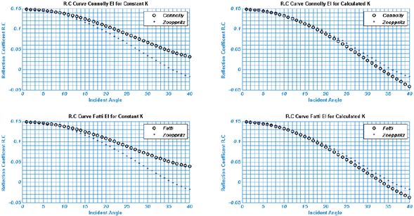
Figure 1 Reflection coefficient curves AVO type I using Connolly and Fatti elastic impedance equations with constant and calculated value of Κ.
For AVO type I when Κ = 0.25, the plot between reflection coefficients derived from Zoeppritz approximation and both elastic impedance equations from Connolly and Fatti start with a similar trend. The curves start to deviate from each other from 10° and continue to deviate as they go towards far angles. By the time the curve reaches 30° both the curves have clear space among them. It is evident from the figures that at far offsets the separation of curves is prominent.
The reflection coefficient is generated using calculated Κ =0.3393 using Equation 6, and the plot between both the reflection coefficient starts with a similar trend and matches correctly. Both the curves begin to deviate from each other from 30°, and the deviation is slight.
AVO Type II
AVO type II shows in figure 2 the reflection curves using Connolly elastic impedance equation for the constant and calculated value of Κ. It starts from near to zero reflection coefficient and the trend is more negative with the increase in the angle. Both curves begin to deviate from each other from 10° and continue to more negative as they go towards the far angles when the constant value of Κ is used. Connolly reflection coefficient curves match mostly but show slight separation as illustrated in figure 3.
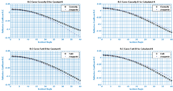
Figure 2 Reflection coefficient curves AVO type II using Connolly and Fatti elastic impedance equations with constant and calculated value of K.
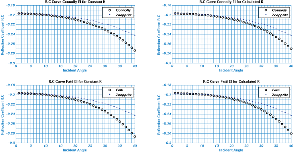
Figure 3 Reflection coefficient curves AVO type III using Connolly and Fatti elastic impedance equations with constant and calculated value of Κ.
When calculated Κ = 0.32395 is used, it was noticed that the elastic impedance curves become more negative than the Zoeppritz curve. Both elastic impedance curves closely match the Zoeppritz reflection coefficient curve.
AVO Type III
The elastic impedance reflection coefficient curve for AVO Type III gives a peculiar behavior for both constant and calculated value of Κ. The deviation of reflection coefficient curves of Zoeppritz and the elastic impedance is similar, and it increases with the angle. As the estimated value of Κ is 0.28921, very close to Κ constant 0.25, Connolly and Fatti elastic impedance equations are only valid up to 20° for both constant Κ and calculated Κ.
AVO Type IV
Type IV is gas sands for which reflection coefficients decrease with increasing offset figure 4. They are noticeable when the S-wave velocity in the gas sand is lower than in the overlying shale(John P. Castagna & Swan, 1997). The reflection coefficient curves for Connolly and Fatti based elastic impedance equations tends to deviate from the Zoeppritz curve from 10 while using Κ = 0.25. While when the calculated Κ 0.3432 is used, the deviation starts from ° 27 for both equations.
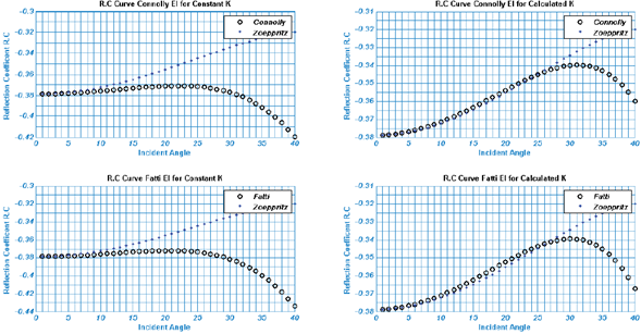
Figure 4 Reflection coefficient curves AVO type IV using Connolly and Fatti elastic impedance equations with constant and calculated value of Κ.
From the results, it can be seen that the value of Κ is a significant factor in elastic impedance inversion and its variation also affects the results. AVO type I and type II give excellent agreement with the Zoeppritz when calculated Κ is used. AVO type III, on the other hand, does not change with the change in the value of Κ. With computed Κ type IV agrees with the Zoeppritz equation until the angle of 27°; this happens when the value of Κ becomes significant upon the use on a considerable scale. So, for a constant value of Κ, the results are good for the near-offset data, but an accurate shear wave and density information from using near-offset cannot be gotten. Thus, it can be deduced that if the calculated value of Κ is used, a good agreement at far offset will give good control over a shear wave and density information. There exists a contradiction which can be resolved using calculated value of Κ. AVO type I and type II will give better results with calculated Κ even at far offsets. While AVO III is more accurate at near angles for constant and calculated Κ. Type IV has a range from close offset for constant and near to mid offset for an estimated value of Κ and these are more accurate at near angles Table 2.
Application of the Well data
The present study has been tested using 70-meter part of well log X in the study area. figure 5a shows the comparison of the well-logs with P-Impedance, and S-impedance, P-wave velocity, S-wave Velocity, and density. The inverted P-Impedance, S-Impedance, P-wave velocity, S-wave velocity, and density is shown as Ip1, Is1, Vp1, Vs1, and p1. Results are generated using Fatti's three-term elastic impedance inversion for the angle gathers with 5% noise. The error in the real and inverted value is shown in figure 5b. It is evident that when Κ constant is used, the inverted logs deviate more from the normal well-logs.
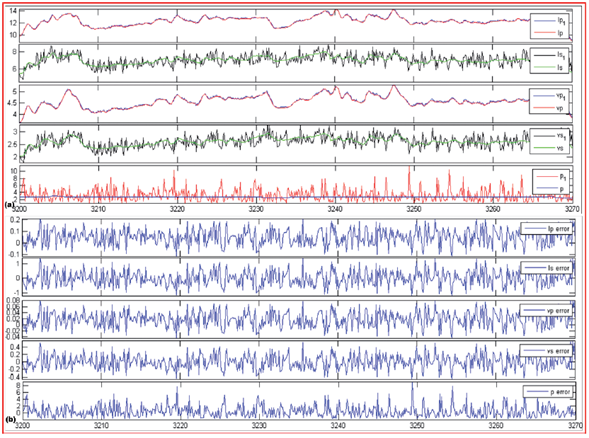
Figure 5 (a) Real and inverted logs P-impedance S-Impedance P-wave, S-wave and Density logs using a constant value of Κ. (b) Error in the real an inverted logs.
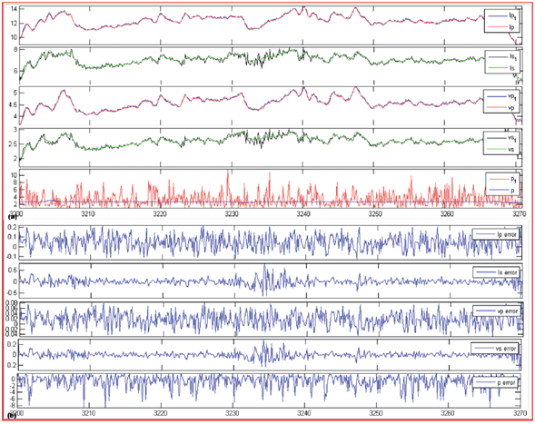
These errors arise because the constant Κ, as Κ = 0.25, or average Κ of well-log data has been taken; it means each layer has the same value of Vs2/VP2. When some segments deviate from this assumption, significant errors are introduced into inversion. The inverted and real curves using the calculated value of Κ are shown in figure 6a. When calculated Κ is used, it is noticed that the error in S-impedance and S-wave velocity is reduced considerably, while in P-impedance and P-wave velocity error is also reduced to some extent as seen in figure 6b. Density in both cases is very unstable while inverting. It gives large errors even for the slight presence of noise. These results agree with the findings that Κ is a significant factor in the interpretation of data in Elastic Impedance Inversion, and it should not be considered as a constant value. The calculation of elastic impedance log is a significant step towards the elastic impedance inversion of seismic data. If the elastic impedance logs are not generated with proper care, it can deprive us of some valuable information in the interpretation of data.
Conclusions
Elastic impedance equations coupled with the Zoeppritz equation can successfully be utilized to identify lithological reservoirs as well as AVO classes. The value of elastic impedance equations constant Κ and its impact on AVO classes and computed reflection coefficient curves were discussed and analytical studied. Sometimes, a fixed value of constant Κ generates an error in lithological reservoirs characterizations. The constraint Κ value was successfully applied to study AVO classes. Results indicate that it improves the matching with Zoeppritz curve to near, mid and far angle for AVO type I and II, and near and mid-offset for AVO type IV. AVO type III does not show significant change with the change in the value of Κ. The decrease in the percentage of error in the inversion of the well's logging segment using calculated value of Κ also agrees with the findings. Thus, it can be induced the findings that keeping Κ constants would give errors in the results, but it is necessary to have proper control over the value of Κ to make the results accurate