Inglês (pdf)
 Artigo em XML
 Referências do artigo
 Enviar este artigo por email
 Citado por SciELO
  Citado por Google
  Similares em
SciELO
Similares em
SciELO  Similares em Google
 Permalink
Introduction
The design of some geotechnical structures requires the estimation of the hydraulic conductivity on soils. Sand-clay mixtures are one of the most common soils involved in these structures, either as the surrounding natural soil, or as fill material. For both cases, the estimation of the hydraulic conductivity allows to quantify infiltration flow rates, infiltration forces, duration of consolidation, among others. The literature shows that for saturated sand-clay mixtures, the hydraulic conductivity depends on the relative proportions between the two materials (Yang & Aplin, 1998; Schneider, Flemings, Day-Stirrat, & Germaine, 2011; Indrawan, Rahardjo, & Leong, 2006; Shafiee, 2008; Shakoor & Cook, 1990; Shelley & Daniel, 1993), the overall density or porosity (Alyamani & Sen, 1993; Chapius, 1990; Hazen, 1911; Kenney, Lau, & Ofoegbu, 1984; Loudon, 1952; Odong, 2007), the mineralogy or material type (Deng, Wu, Cui, Liu, & Wang, 2017) and the interconnection between pores (Belkhatir, Schanz, Arab, & Della, 2014).
A vast number of correlations to estimate the hydraulic conductivity has been proposed depending on the mentioned properties. Authors report correlations to estimate the hydraulic conductivity of clean sands (Amer, Asce, Amin, & Awad, 1974; Biernatowski, E. Dembicki, Dzierzawski, & Wolski, 1987; Kollis, 1966; Pazdro, 1983), clean clays (Mesri & Olson, 1971; Al-Tabbaa & Wood, 1987; Nagaraj, Pandian, & Raju, 1994; Samarasinghe, Huang, & Drnevich, 1982; Tavenas, Leblond, Jean, & Leroueil, 1983), kaolin clays (Mesri & Olson, 1971; Hamidon, 1994), and sand-clay mixtures (Chapius, 1990; Kenney, Van Veen, Swallow, & Sungaila, 1992; Kumar, 1996; Shafiee, 2008; Luijendijk & Gleeson, 2015).
Correlations for the estimation of hydraulic conductivity are mostly calibrated on experimental results using homogeneous soil samples (Al-Tabbaa & Wood, 1987; Amer, Asce, Amin, & Awad, 1974; Biernatowski, E. Dembicki, Dzierzawski, & Wolski, 1987; Chapius, 1990; Kollis, 1966; Kumar, 1996; Mesri & Olson, 1971; Nagaraj, Pandian, & Raju, 1994; Pazdro, 1983; Samarasinghe, Huang, & Drnevich, 1982). To achieve homogeneity, for example in sand-clay mixtures, researchers often mix the two different materials by hand, until a homogeneous soil mass is obtained (Koltermann & Goerlick, 1995; Revil & Catchles, 1999). Disappointingly, the reality shows something different: the experience tells us that samples obtained in a single layer of a sand-clay soil, present similar (but not equal) fine content with a certain dispersion (Gomez-Hernandez & Gorelick, 1989; de Dreuzy, de Boiry, Pichot , & Davy, 2010). In the geotechnical practice, the mean value of fine content is often used to classify the mixed soil of a single layer, and with this, some properties such as the hydraulic conductivity are estimated. This suggests that the influence of the spatial distribution of the fine content is in some soil properties disregarded. This fact is disappointing considering the existing numerical tools which allow to investigate this influence (Dassault Systèmes, 2016). Definitely, more investigation is in this direction recommended.
In this work, the influence of the spatial distribution of the fine content in sand-clay mixtures is investigated. For this purpose, some experiments are conducted to study the behavior of the hydraulic conductivity of a sand-clay mixture. Characterization tests and permeability tests are systematically performed to that end. A Kaolin clay and the Santo Tomas sand are mixed with different proportions to obtain sand-clay mixtures. The hydraulic conductivity results are carefully examined to calibrate an exponential regression curve. Having this, the influence of the spatial distribution of the fine content is investigated through numerical simulations. A Boundary Value Problem with finite elements is constructed simulating a constant head hydraulic conductivity test with large sample dimensions. For the proposed model, different spatial distributions of the fine content are considered following a Gaussian distribution. The influence of the Gaussian distribution parameters, namely the mean value and the standard deviation, is carefully studied. At the end, a Boundary Value Problem of a flow around a sheet pile wall is simulated for comparison purposes. Finally, some concluding remarks are given.
Material characterization
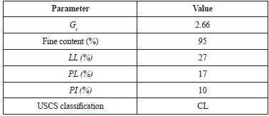
In this section, the testing soils are characterized. A set of experiments including sieve analysis, hydrometer analysis, specific gravity and Atterberg limits have been conducted on these materials. The testing clay corresponds to a Kaolin clay from the northern region of Colombia. Similarly, the testing sand corresponds to the Santo Tomás sand, very often used for construction purposes in Colombia. Characterization tests have been conducted on the Kaolin clay with the following results. It presents a specific gravity of G s = 2.66, a fine content (percent passing sieve #200) of 95%, a liquid limit of LL = 27%, a plastic limit of PL = 17% and plasticity index of PI = 10% According to the Unified Soil Classification System USCS, the Kaolin clay is classified as a low plasticity clay CL. Results are summarized in Table 1.
Table 1 Characterization test results of the Kaolin clay. G s : specific gravity, LL: liquid limit, PL: plastic limit, PI: plasticity index.
The Santo Tomás sand is a uniform sand with a fine content of 1.21%, uniformity coefficient of C u = 4.08, curvature coefficient of C c = 0.98, effective diameter of D 10 = 0.16 mm, specific gravity of G s = 2.65, maximum void ratio e max = 0.91 and minimum void ratio e min = 0.54. The latter values are related to maximum and minimum dry densities of ρ dmax = 1.72 g/cm3 and p dmin = 1.39 g/cm3 respectively. According to the Unified Soil Classification System USCS, the Santo Tomás sand is classified as a poorly graded sand SP. The results are shown in Table 2. The grain size distributions for the Santo Tomás sand and the Kaolin clay, obtained by sieve analysis and hydrometer analysis respectively, are shown in Figure 1.
Table 2 Characterization test results of the Santo Tomás sand. G s : specific gravity, D 10: effective diameter, C u.uniformity coefficient, C c : curvature coefficient, e max : maximum void ratio, e mln : minimum void ratio
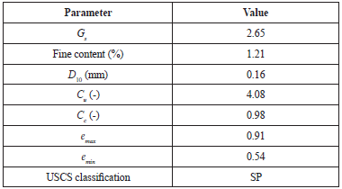
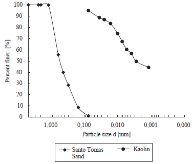
Figure 1 Grain size distribution for Santo Tomás sand and the Kaolin clay. Test method: sieve analysis for Santo Tomas sand, hydrometer analysis for Kaolin clay.
Results of hydraulic conductivity tests of the sand-clay mixtures
A number of permeability tests were conducted on the different testing materials, namely the Santo Tomás sand, the Kaolin clay, and the sand-clay mixtures with different proportions. Constant head permeability tests were conducted on all samples (INVIAS, 2013), except for the one of the Kaolin clay, in which considering its low hydraulic conductivity, a variable head permeability test was performed. Samples were prepared with initially ovendried Santo Tomas sand and dried Kaolin clay powder. A small amount of water was mixed thoroughly until reaching a homogeneous soil mass with a water content of approximately w ≈ 10% The process of homogenization was performed by hand on an external recipient. The wet tamping method, with three layers of approximately 2.0 cm, was used to produce samples within the permeameter. The followed procedure was as follows: for the first layer, the permeameter cell was filled with 2 centimeters of water. Then, the soil was gently poured till reaching approximately half centimeter above the water surface. A special cylindrical tamper with diameter of 5 cm was used to compact the first layer, by providing 25 blows on the surface. The procedure was repeated for the second and third layer. Special care was taken by controlling the blow intensity and by keeping the number of blows constant, in order to produce samples with similar (but not equal) void ratios. The void ratio for the clean sand sample was e = 0.72 which corresponds to a relative density of D r = 51.3% (medium dense sand) and a dry density of ρ d = 1540 kg\m3 For the case of mixed sand-clay samples, void ratios within the range of e = {0.65 - 0.72} were always obtained, corresponding to dry densities of ρ d = {1610 - 1540} kg\m3 The void ratios were always checked at the end of the preparation process, and in case that the resulting one was not within the expected range, the procedure was then repeated. Top and bottom porous stones, covered by filter papers were included in the assembly. A standard spring for permeameters was fixed on the top porous stone to provide a small vertical stress to all samples (Bardet, 1997). Then, the sample was continuously flooded with distilled water during two days to guarantee its complete saturation (degree of saturation equal to one). Detailed description of the followed test procedure can be found in the literature (Bardet, 1997; INVIAS, 2013).
The prepared sand-clay mixtures include fine contents of {0%, 4%, 8%, 12%, 16%, 20%, 100%}. The case of 0% corresponds to clean Santo Tomas sand (without fines), and 100% to clean Kaolin clay. The results of the hydraulic conductivity tests are compiled in Table 3, including a correction due to temperature according to the method by (INVIAS, 2013).
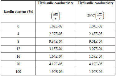
A suitable exponential interpolation function depending on the fine content FC is employed to adjust the results, which considers the hydraulic conductivity of clay, denoted by k 100, and the hydraulic conductivity of clean sand, denoted with k 100 and read

Where c is a material constant to be calibrated. Notice that for FC = 0, the proposed relation renders k = k0, while for FC = 100, a value of k ≈ k 100 is obtained. For the reported results, a value of c = 0.28 has been found to reproduce well the observed behavior. Figure 2 includes the experimental results in conjunction with the proposed relation, and an accurate estimation.
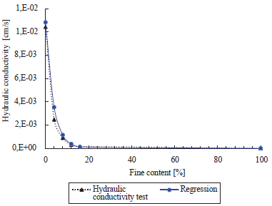
Figure 2 Results and adjusted regression of hydraulic conductivity test for different fine contents (T=20°C)
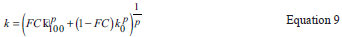
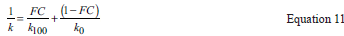
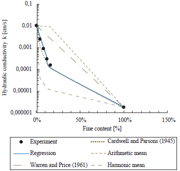
Figure 3 plots once more the obtained results of the permeability tests, and compares it with the adjusted regression and other correlations reported in the literature for sand-clay mixtures. It includes the relation by (Warren & Price, 1961), (Cardwell & Parsons, 1945), and others as the arithmetic mean and harmonic mean as a function of the fine content FC. A brief summary of these relations is given in Appendix B, while their analysis may be found in other works, e.g. (Luijendijk & Gleeson, 2015). Notice that the relation by (Cardwell & Parsons, 1945) includes parameter , which must be adjusted. The cases p = 1 and p = -1 correspond to the arithmetic and harmonic means respectively. For the particular correlation by (Cardwell & Parsons, 1945), it has been found that a value of p = -0.4 matches well the obtained results. The fact that parameter p is lower than zero, indicates that the hydraulic conductivity is mostly dominated by the clay portion (Luijendijk & Gleeson, 2015).
Numerical simulations to evaluate the effect of the spatial distribution of the fine content on the equivalent hydraulic conductivity
For a non-homogenous soil sample, i.e. a sample presenting spatial variations of the fine content and/or other variables, the equivalent hydraulic conductivity k eq is the one resulting from the homogenization of a representative volume. With simpler words, if we perform a constant head hydraulic conductivity test, the equivalent hydraulic conductivity k eq is the one resulting from the test, independently of the sample inner heterogeneities. In this section, the influence of the fine content heterogeneity is evaluated through numerical simulations. For that end, Boundary Value Problems BVPs with finite elements are constructed. The BVPs simulate sand-clay mixtures subjected to a steady state water flow. The simulations account for spatial distributions of the fine content with a certain statistical distribution. Details of the creation of this heterogeneity will be explained later on. With this procedure, different points within the problem may have different fine contents and therefore different hydraulic conductivities. The hydraulic conductivity has been correlated to the fine content according to Equation 1. The results will show whether the equivalent hydraulic conductivity resulting from the overall problem depends or not of the fine content spatial distribution.
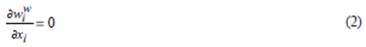
The BVPs assume 2D conditions under plane strain assumptions. The commercial software Abaqus Standard V6.16 (Dassault Systèmes, 2016) is used for these simulations. The simulations are based on the steady state equation for underground water flow, which using indicial notation reads:
where x i ={x 1 ,x 2} are the coordinates and w i w is the Darcy flow velocity vector defined as:
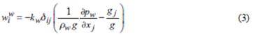
where ô ij is the Kronecker delta operator, k w is the hydraulic conductivity coefficient, p w is the water pore pressure, p w is the water density, g is the gravity magnitude and g. is the unit vector pointing in the gravity direction. The hydraulic coefficient K can be also related to the material's permeability k through the relation k = K (μ / p w g), where μ is the dynamic viscosity of the fluid. Notice that we have considered isotropic hydraulic conductivity. Steady state analysis of groundwater flow does not depend on the material's mechanical behavior, and therefore no constitutive model for the soil is in the present analysis required.
Different spatial distributions of fine content are considered for the analysis. Specifically, random values of fine content saved at each element Gauss point are simulated. These values follow a Gaussian distribution with mean value  and standard deviation
  . Variation of these variables {
 ,} were considered for the analysis, including the fine content mean values of 2.0%, 5% y 10%} and standard deviations computed as a fraction of the mean value, i.e. σ = F, where F takes different values between 0 and 1.
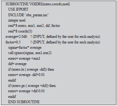
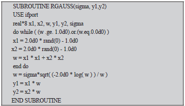
The non-homogenous fields of fine content were simulated through a special FORTRAN subroutine (INTEL(R) , 2007) compatible with ABAQUS. The software provides the user subroutine VOIDRI which enables to create an initial field, usually the void ratio, and permits to establish a direct relation between this variable and the hydraulic conductivity. Hence, we have used this user subroutine to write a FORTRAN code able to produce a random value for the fine content following the aforementioned Gaussian distribution. The code is given in Appendix A. The subroutine inputs correspond to the mean value and standard deviation a, which are controlled for each simulation.
Three different Boundary Value Problems BVPs were constructed: the first simulates a constant head hydraulic conductivity test with a large soil simple, with dimensions of 1 m times 1m. This BVP allows to compute an equivalent hydraulic conductivity for a given heterogeneous field of fine content. The second corresponds to the same problem under the three-dimensional (3D) case. The last problem simulates a bidimensional flow around a sheet pile. In the following lines, a brief description of the problems is given and their results are carefully analyzed.
Simulation of a constant head hydraulic conductivity test with heterogeneous soil
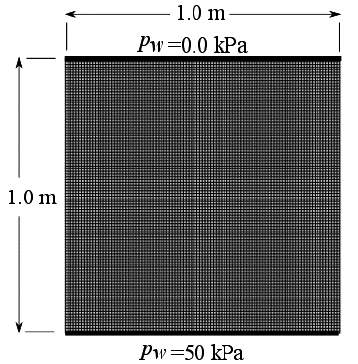
The simulation considers a squared domain of a large soil sample, with dimensions of 1 m wide times 1 m high. The aim is to simulate the test depicted in Figure 4, wherein a vertical upward flow is experienced by the soil due to an imposed hydraulic gradient. Small sized finite elements were used (of 0.01 mx 0.01 m) for the BVP. At the top boundary, a pore water pressure equal to p w = 0 kPa is fixed as boundary condition to allow its drainage. At the bottom, a water pressure of p w =50.0 kPa is given to produce the pressure differential. The geometry, mesh and boundary conditions are depicted in Figure 5.
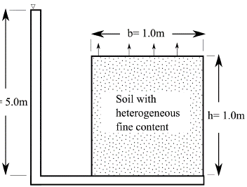
Figure 4 Schematic model of hydraulic conductivity test. The model geometry is not scaled. The water flows upward.
The developed FORTRAN subroutine, described in the previous section, was used to generate the random field of fine content following a Gaussian distribution. As an example, Figure 6 presents the fine content contours for a mean value of µ = 5% and standard deviation of = F× = 0.5x5%
= 2.5%.
= 0.5x5%
= 2.5%.
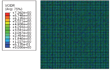
Figure 6. Simulation of hydraulic conductivity test. Random field of fine content with mean value of µ = 5% and standard deviation of =FX = 0. 5x5% = 2.5%.
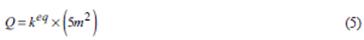
The computation of the equivalent hydraulic conductivity is as follows. According to the Darcy's law (Darcy, 1856), the water outflow Q obtained at the top boundary is computed with:

where k eq is the equivalent hydraulic conductivity, i = ∆h / H is the hydraulic gradient, ∆h is the water head differential, H is the height of the sample and A is the transversal section area of the sample. For the given geometry, ∆h = 50kPa / y w = 5m, H=1 m and A = 1m x 1m. Substitution of these values yields to the following simpliied relation:
On the other hand, the flowrate is computed with: ,

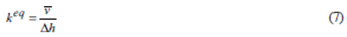
where  is the mean velocity of the water outflow. The latter is simply computed by averaging this variable at the top boundary nodes. Substitution of Equation 6 in Equation 5 yields to the following relation for the equivalent hydraulic conductivity:
Results of simulations for mean fine contents of = {5%,10%} with different values of the standard deviation a are plotted from Figure 7 to Figure 12. Figure 7 presents the resulting outflow velocity v for each node located at the top boundary for = 5%. As expected, scattered values of the outflow velocity v are obtained due to the fine content heterogeneity. Notice that the dispersion increases for higher values of F, where F is the factor controlling the standard deviation σ = F, see Figure 7. The resulting mean outflow velocity, denoted by v, is plotted in Figure 8. It is reminded that the mean outflow velocity results from averaging the outflow velocities v. The results clearly indicate an increasing behavior of the mean outflow velocity v for increasing values of F. The resulting equivalent hydraulic conductivity keq, computed with Equation 7, is plotted in Figure 9 and presents the same trend. Hence, one may conclude that the equivalent hydraulic conductivity keq depends on the spatial distribution of the fine content. Similar results were obtained for a mean fine content of = 10% as shown in Figure 10, Figure 11 and Figure 12.
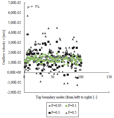
Figure 7 Outflow velocity at the top boundary nodes. Mean fine content of = 5%. The standard deviation is computed as σ = F×, where F is a factor. BVP of hydraulic conductivity test.
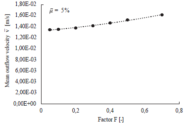
Figure 8. Mean outflow velocity vs. factor F. Mean fine content of = 5%. The standard deviation is computed as σ = F×, where F is a factor. BVP of hydraulic conductivity test.
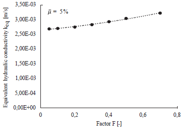
Figure 9 Equivalent hydraulic conductivity vs. factor F. Mean fine content = 5%. The standard deviation is computed as σ = F×, where F is a factor. BVP of hydraulic conductivity test.
⅛5
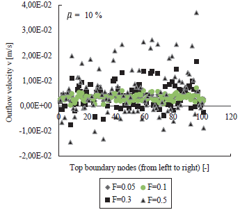
Figure 10 Outflow velocity at the top boundary nodes. Mean fine content of = 10%. The standard deviation is computed as σ = F×, where F is a factor. BVP of hydraulic conductivity test.
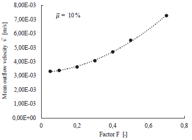
Figure 11 Mean outflow velocity vs. factor F. Mean fine content of = 10%. The standard deviation is computed as σ = F×, where F is a factor. BVP of hydraulic conductivity test.
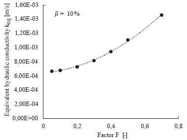
Figure 12 Equivalent hydraulic conductivity vs. factor F. Mean ine content of = 10%. The standard deviation is computed as σ = F×, where F is a factor. BVP of hydraulic conductivity test.
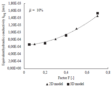
We are now interested to extend the analysis for the three dimensional (3D) case. For this purpose, a 3D FE-model has been constructed. The geometry consists of a cube of 1m x 1m x 1m. While displacements are in all directions restricted, a pore pressure gradient is similarly produced by imposing a value of 50 kPa at the bottom, and 0 kPa at the top. The random field of fine content is generated in the same way as in the 2D model. Figure 13 shows an example of the fine content FC heterogeneity for the mean value of µ =10% and standard deviation of µ = 4%. Figure 14 shows the results for the equivalent hydraulic conductivity k eq of the 2D and 3D models, whereby very small discrepancies are observed. Hence, one may expect very similar conclusions on the 3D case.
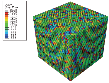
Figure 13 Simulation of hydraulic conductivity test, 3D FE model. Random field of fine content with mean value of µ =10% and standard deviation of = F× = 0.4x10% = 4%
Simulation of a flow around a sheet pile wall with heterogeneous soil
The influence of the fine content heterogeneity is now analyzed in a simulation of a water flow around a sheet pile. Similar to the previous simulations, a distribution of the fine content is given following a Gaussian distribution. The sheet pile wall is submerged in the soil with a depth of 3 m and a thickness of 0.2 m, as depicted in Figure 15. The problem is 20 m wide and 6 m high. Lateral and bottom boundaries are considered as impervious. The sheet pile itself is considered as impervious as well. In order to generate a water flow around the sheet pile, a water pressure of P w = 0 kPa is fixed on the left top boundary, while a water pressure of p w = 100 kPa is set on the right top boundary. The geometry, mesh and boundary conditions are depicted in Figure 15.
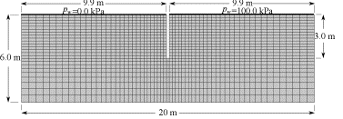
Figure 15 Mesh, geometry and boundary conditions for BVP of a sheet pile wall. Water flows around the sheet pile, from the left side to the right side.
As an example, the spatial distribution of the fine content for a mean value of  = 5% with a factor of F = 0.9 is plotted in Figure 16. The figure shows the initial heterogeneity of the fine content.
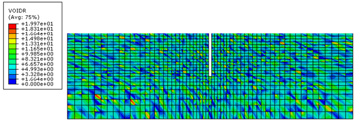
Figure 16 Spatial distribution of the fine content for a mean value of 5% and a factor of F = 0.9. The standard deviation is computed as σ = F×, where is a factor. BVP of flow around sheet pile wall
The contours of the pore water pressure are shown in Figure 17 and the excess of pore water pressure, computed as ∆pw = p
w
- p
w0
, where P
w0
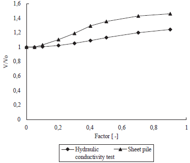
is the initial pore water pressure, is plotted in Figure 18. In general, these plots show the typical flow net of a water flow around a sheet pile wall. Once more, the nodal outflow velocities, from the left top boundary, are plotted in Figure 19. The results show that for nodes closer to the sheet pile, the outflow velocity increases. Dispersion is again obtained in these results due to the heterogeneity of the fine content. Their mean values are plotted in Figure 20 and similar to the hydraulic conductivity test simulation, it shows an increasing behavior for increasing standard deviation. For comparison purposes, we have now plotted in Figure 21 the response of the normalized velocity  /0, where 0 is the velocity for the homogeneous case σ = 0, for a mean fine content of = 5%. Surprisingly, both results show a similar response despite they were computed on very different Boundary Value Problems.
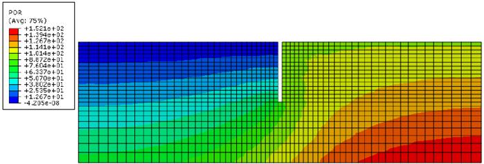
Figure 17 Contours of pore water pressure p
w
. Mean fine content of  = 5% and F = 0.9. The standard deviation is computed as σ = F×. BVP of flow around sheet pile wall
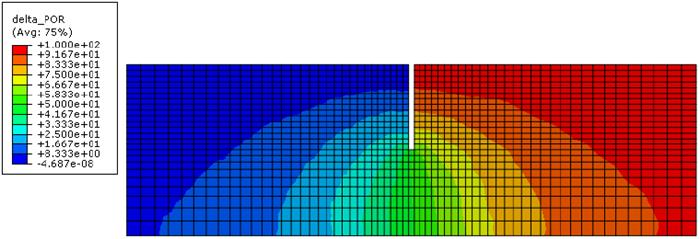
Figure 18 Contours of excess of pore water pressure ∆p
w = p
w
- P
w0
, where p
w0 is the initial pore water pressure. Mean fine content of = 5% and F = 0.9. The standard deviation is computed as σ = F×. BVP of flow around sheet pile wall
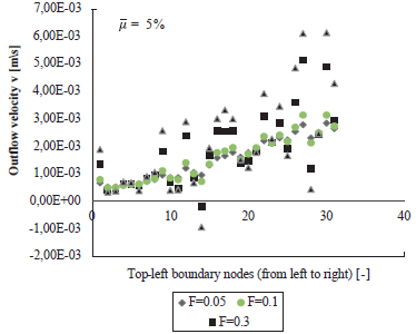
Figure 19 Outflow velocity at the top left boundary nodes. Mean fine content of = 5%. BVP of flow around sheet pile wall
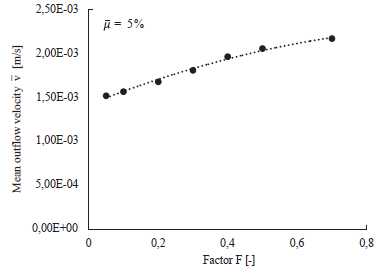
Figure 20 Mean outflow velocity vs. factor F. Mean fine content of  = 5%. The standard deviation is computed as σ = F×, where F is a factor. BVP of flow around sheet pile wall

Final remarks
In the present work, the influence of the fine content heterogeneity on the hydraulic conductivity was evaluated. For this purpose, a set of FE simulations of a large scaled permeability test with constant head was performed. The simulations considered the behavior of the hydraulic conductivity of the Santo Tomas sand, mixed on different proportions with a Kaolin clay, according to some experiments. The results showed a clear dependence of the resulting equivalent hydraulic conductivity with the spatial distribution of the fine content. Specifically, it was shown, that for a given mean fine content, increasing standard deviations a are related to higher equivalent hydraulic conductivity values keq. This trend is at least true for mean values of fine contents of µ = {5%.10%} for the FE models tested in the present work. Of course, additional simulations are required to analyze the resulting trend on a larger range of mean fine content.
The results suggested that spatial variability of the fine content should be considered in Boundary Value Problems for a more realistic response. The last fact was demonstrated with the simulation of a water flow around a sheet pile which showed a similar pattern in the results. Currently, more investigation is made to validate the numerical results with experiments on large scaled samples considering their heterogeneity.