


 Inglês (pdf)
 Artigo em XML
 Referências do artigo
 Enviar este artigo por email
 Citado por SciELO
  Citado por Google
  Similares em
SciELO
Similares em
SciELO  Similares em Google
 Permalink
Introduction
Landslide risk analysis is inherently complex. The greater difficulties in achieving reliable results for landslides in comparison with other natural threats, such as earthquakes and floods, have been highlighted in the literature. Such difficulties are due to the complexity of modeling landslide hazard, intensity and the vulnerability of the built environment to landslides (Uzielli et al., 2008).
The concept of vulnerability is often related to the degree of loss of an element suffering damage during the interaction with an external force of a given intensity (Hollenstein, 2005; Uzielli et al., 2008; Fuchs, Heiss, and Hubl, 2007; Unesco, 1979). Some other definitions and related concepts have been studied in several technical publications. Thus, the terminology is sometimes frustrating and even confusing as visible in the paper by Nicu (2016) where the concept of vulnerability is associated to a semi-quantitative index that represents a measure of the exposure of a population to some hazard; the index is a composite of five quantitative indicators properly combined via AHP (Analytic Hierarchic Process) to obtain a numerical result. In this case, it is clear that exposure is proposed as synonymous of vulnerability which differs from some classical papers (Li et al, 2010; Fell et al., 2005) where the exposure (E) is a measure of the probability of physical interaction between the hazard and the vulnerable (V) element (people, buildings, environment, infrastructure). Once the interaction is materialized, a consequence (C=VxE) came to appear in the form of economic/environmental/societal loss.
The external force represents a natural phenomenon (hazard) that may be characterized in terms of temporal, spatial and magnitude probabilities. The effects of the interaction between the hazard and the exposed element depend on the intensity of the hazard, which may be defined as "a set of spatially distributed parameters describing the destructiveness" of the hazard process (Hungr, 1995) and, alternatively, on the resistance, which sometimes is called susceptibility, of the element at risk, which describes the propensity of a building or other infrastructure to suffer damage from the impact of a specific hazard (Li et al., 2010) vulnerability is widely accepted to be defined as the degree of loss (or damage. Consequently, a modern concept of vulnerability must consider not only the intensity of the hazard but also the structural resistance of the exposed infrastructure. This concept is referred to as physical vulnerability, and the most accepted definition, per (Fell et al., 2005), is a representation of the expected degree of loss quantified on a scale of 0 (no damage) to 1 (total destruction). Thus, a vulnerability assessment requires an understanding of the interaction between the hazard and the exposed element. This interaction can be expressed using empirical vulnerability curves (Quan Luna et al., 2011), mathematical - decisional models (Pascale, Sdao, and Sole, 2010), heuristic rules (Birkmann et al., 2013), physical vulnerability curves (Kang and Kim, 2015), quantitative vulnerability functions (Fuchs, Heiss, and Hübl, 2007), expert knowledge systems (Bell and Glade, 2004; Zêzere et al., 2008), numerical modeling (Llano-Serna, Farias, and Martínez-Carvajal, 2015) and quantitative estimation of vulnerability that are based on scenarios that consider different kinematic intensity models (Li et al., 2010).
From the natural science perspective, vulnerability assessment can be split into two main procedures, which require different methods and assumptions: estimation of the vulnerability of life and vulnerability of property. Despite its importance, defining the potential fatalities has not been intensely considered in landslide risk management, perhaps due to the intrinsic difficulty of its objective definition (Bell and Glade, 2004). Only recently, some authors have approached the problem, largely relying upon considerations on the host structures and infrastructure, population census data such as density, education level or average age (Liu and Lei, 2003) or consequence analysis (Uzielli et al., 2008).
Previous studies about landslides and debris flows have mainly focused on landslide hazard assessment and the corresponding triggering mechanisms (Jaiswal, van Westen, and Jetten, 2010; van Westen, Rengers, and Soeters, 2003). However, there is an increasing interest in research on risk assessment (Totschnig and Fuchs, 2013; Nicu, 2018). For a risk assessment, vulnerability assessment is required for the elements at risk during landslide/flow.
As stated in (Mergili et al., 2012), the term debris flow does not always refer to exactly the same process. Some authors consider it a landslide with a fluid-like motion (Corominas et al., 2003; Mergili et al., 2012), others consider it runoff with very high sediment concentration (O'Brien et al., 2007). However, these two approaches are not necessarily contradictory- they depend on whether the observer has a geotechnical or a hydrological background. As presented in Figure 1, there are a number of similarities between landslide and debris flow related to the vulnerability assessment. Thus, it is possible to postulate that a unique model, when properly defined, may consider the quantification of the physical vulnerability for both processes.
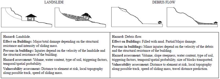
Figure 1 Schematic representation of landslide and debris flow damages related to the location of the elements at risk in relation to the hazard. Modified from (van Westen, van Asch, and Soeters, 2006).
The main objective of this paper is to present a physical vulnerability model for diverse types of structures to allow a quantitative assessment of landslide/debris flow risks. Additionally, the vulnerability function is characterized according to the structural resistance of the buildings and their spatial location in relation to the hazard position. The proposed model has potential applications in regional quantitative assessment of the physical vulnerability of buildings to landslide and debris flow events.
Vulnerability framework
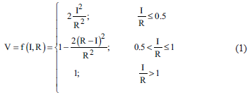
According to (Li et al., 2010), vulnerability depends on both the characteristics of the element at risk and the landslide intensity. The abovementioned authors proposed a model in which the vulnerability (V) is analyzed on average as a function of the hazard intensity (I) associated with exposed elements at risk and the resistance ability (R) of the elements to withstand a threat, as presented in Equation 1, where both intensity (I) and resistance (R) is expressed in non-dimensional terms. The intensity may be expressed using any of the next variables or their combinations: velocity of sliding mass, energy, volume and depth of mobilized detritus. As depicted in Figure 1, the quantification of the intensity may be assessed using the velocity, as presented in Equation 2.

where I dyn is the dynamic intensity factor (Eq. 3) and I dpt is the debris-depth factor (Eq. 4).
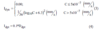
In the previous equations, C represents the averaged velocity (in mm/s) of sliding mass, and Ddpt is the debris depth (in meters) at the building location. Taking into consideration that the methodology must be applied as a planning tool prior to the occurrence of the landslide/debris event, the estimation of the parameters C and Ddpt must be performed using empirical, simplified analytical or numerical simulation methods. Considering that the simplified and empirical methods do not always guarantee the necessary accuracy for most of the applications and that the numerical simulations demand high computational costs, the proposed vulnerability model is difficult to incorporate, at least as a regional tool, in a GIS (Geographic Information System) environment for planning purposes.
Using the creativity of Li's model, a new variable was defined, named T, which is presented in Equation 5 and which was originally proposed by (Guimaraes-Silva 2015).

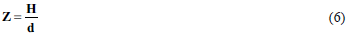
where R represents the structural resistance of the building and Z represents a modified gradient defined in Equation 6.
The extreme values of V are zero and 1. According to Equation 5, the independent variable Z represents the intensity of the landslide process; consequently, it strongly controls the value of the vulnerability. The introduction of variable T is necessary because it considers not only the intensity, but also the structural resistance of the buildings, R. The lower the resistance of the building, the higher the vulnerability.
Figure 2 shows a schematic representation of the topographic variables H and d. It is noticed that d must be measured along the possible track of the sliding mass from the hazard location until the center of the plan area of the building. The measurement of d is straightforward when using the appropriate tools of most of the common GIS software already available.
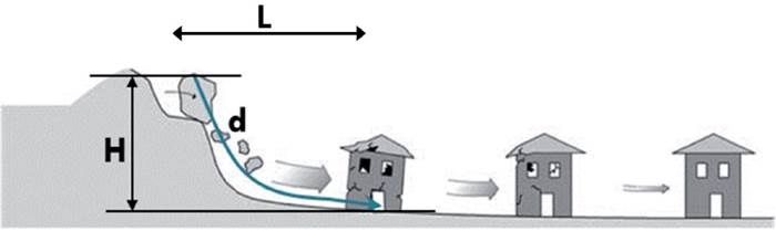
Figure 2 Definition of the topographic variables H and d. Modified from Glade, Anderson, and Crozier, 2005.
Agreeing with Iverson, Logan, and Denlinger (2004), debris flow can be divided into hillslope debris flow (landslides) and channelized debris flow. Hillslope debris flow has a smaller size, short travel distance and faster moving speed compared with channelized debris flow. To understand the type of debris flow, the abovementioned author studied the mobility index of debris as the ratio of the horizontal distance L between the source area and distal limit of the deposit to the difference in height H, which corresponds to the mobility of gravity-driven mass flows. The origin of such approximation is the fahrboschung, tanα=H/L, which is defined by the ratio between the start-stop point elevation difference of the debris (H) and the corresponding horizontal travelled distance (L). The fahrboschung angles range from 21° to 24° for the coarse portion of the debris and from 11° to 14° for the respective fluid portions (Nocentini et al., 2015). In this study, both the mobility index and the fahrboschung were tested as descriptors of the landslide/debris intensity without satisfactory results. The higher the sinuosity of the track of the sliding mass, the poorer the capacity of these variables to properly approximate the landslide intensity.
Finally, the resistance (R) is easily estimated by Li's model, and consequently, it is not necessary to introduce modifications to the original formulation. Thus, Equation 7 may be used directly.
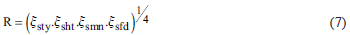
where ξsty, ξsht, ξsmn, and ξsfd are the resistance factors of the structure type, height, maintenance state and foundation depth, respectively. These factors are comprehensively enlightened, and their values are presented in Li et al. (2010).
Theoretical background for the T-Model origin
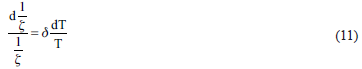
According to Juarez-Badillo (1985), all natural phenomena have a quality of beauty, which means that they are ordered and simple. The quality of order means that these phenomena may be described using mathematical equations. On the other hand, the quality of simplicity means that the referred equations are harmonic. In this context, harmony means that the equations must be complete and symmetrical. Appropriate variables are those that are capable of describing the phenomena in the simplest way possible. For example, for a defined change in volume in a soil mass, the volume (V) together with the variable (1+e) are the appropriate variables, whereas the void ratio (e) wouldn't be by itself.
Consider a phenomenon that is described by the appropriate variables x and y in such a way that y=y(x) with x being in the real domain from zero (0) to infinite (∞). If for a set of extreme values of y, y0=y(0) and y∞=y(∞), then the real domain of y is not complete. Then, consider ζ=ζ(y) the appropriate function of y with a complete real domain, and this is ζ(y0)=0 and ζ(y∞)=∞.
There are two complementary basic principles:
The equation that relates y and x may exist uniquely through a non-dimensional parameter and must satisfy the boundary conditions y0=y(0) and y∞=y(∞) independently of critical points.
The relationship between y and x may exist merely through the appropriate function ζ, and it must possess a satisfactory non-linear proportionality, as shown in Equation 8.
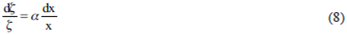
where α is the proportionality dimensionless parameter.
Equation 8 defines an appropriate non-linear proportionality between y and x through the function ζ = ζ (y), which is presented in Equation 9.
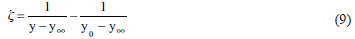
where y∞< y0
Note that in Equation 9, ζ(y0)=0 and ζ(y∞)=∞. Additional details about the philosophical conception of this procedure are presented in Juarez-Badillo (1985), where the author uses the code, named “Principle of Natural Proportionality”, to obtain general equations for describing stress-volume-time and stress-strain behavior of geomaterials, explain common geotechnical problems as settlements, consolidate clayey soils and cyclic behavior of granular soils, among others.
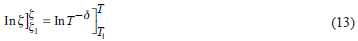
Returning to the previously presented vulnerability model, it is noticeable that the phenomena that describe the interaction between the sliding mass (landslide/debris) and the building are represented using two simple variables: V and T. The real domain of T (Eq. 5) is from 0 to ∞, and consequently, the vulnerability function assumes values in the domain from 0 to 1. In other words, when T is minimum (equal to zero), the vulnerability (V) is zero; on the other hand, when T reaches its maximum theoretical value (∞), the vulnerability is 1. The relationship between these variables, according to the “Principle of Natural Proportionality,” must be stated thorough an “appropriate” function, with a complete real domain between 0 and ∞. Therefore, the functions  and T are the simplest with real complete domains, and consequently, it is possible to verify that when T varies from 0 to ∞, ζ varies from ∞ to 0. The relationship between these appropriate functions must be of the type expressed in Equation 10.
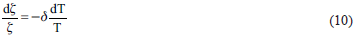
where δ is the proportionality coefficient.
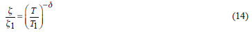
Figure 3 presents a schematic representation of V=f(T) in terms of appropriate variables with a complete real domain. When T varies from 0 to ∞, the variable 1/ζ also varies from 0 to ∞, and thus, Equation 11 can be presented as
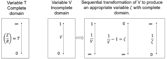
The left term of Equation 11 can be rewritten to obtain
By combining Equation 11 and Equation 12, the initial Equation 10 is obtained, which must be integrated to obtain
where (T1, ζ1) is a knon point that leads us to
From Figure 3, the expression for the variable ζ is introduced in Equation 14 to obtain Equation 15 to Equation 17.
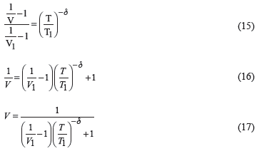
The known point (T1, V1) must be encountered from field observation. Here, it defines T1 as the "characteristic value" of T when V1=0.5, and then, Equation 17 becomes
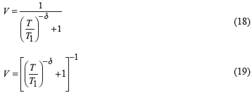
Finally, Equation 19 is the theoretical vulnerability model, where T is the variable previously defined in Equation 5 and δ is a coefficient that governs the average relationship between the sliding mass and the building. The calibration process leads to the determination of the best values for both T1 and δ.
Calibration procedure for the T-Model
To obtain the "characteristic value" T1, a methodology was adopted that is based on the observation of the consequences of several landslides, which occurred in Nova Friburgo, Brazil during the extreme rainfall event on the 11th and 12th of November, 2011.
The catastrophic rainfall produced 1620 landslides in the urban area of Nova Friburgo and more than 7000 landslides in the rural area of the "Serrana Region" that includes the municipalities of Nova Friburgo, Petrópolis, Conselheiro Paulino, Cachoeiras do Macacu and Bom Jardim. Because of the high number of fatalities (more than 1000) and extreme economic losses, this event is currently considered the worst meteorological disaster in Brazil (Entralgo, 2013). Further details on the event itself are presented in Margottini, Canuti, and Sassa, 2013, and Entralgo, 2013.
The calibration procedure involves a three steps methodology where the first step is the analysis of the landslide inventory, then it comes the determination of the parameters T1 and 5; and finally the analysis of the effect of the modified gradient on the theoretical vulnerability. Every one of these steps is detailed presented in next sections.
Landslide Invetory
According to Entralgo (2013), the number of landslides inventoried in "Serrana Region" was 7 268 in an area of 1 217.67 km2 (Figure 4). Because the majority of landslides occurred in rural areas, it was necessary to include the urban area of Nova Friburgo in a polygon where the consequences on buildings and civil infrastructure were more severe (Figure 5). Figure 6 was prepared to show a zoomed area of the selected polygon with the intention of showing an example of the type of landslide and its effect on buildings. The next step was to identify all structures inside the polygon that were affected by landslides and using historical imageries, to make a before-after comparison of damages, as shown in Figure 7. The coordinates datum used in this study was UTD/Datum SIRGAS 2000.
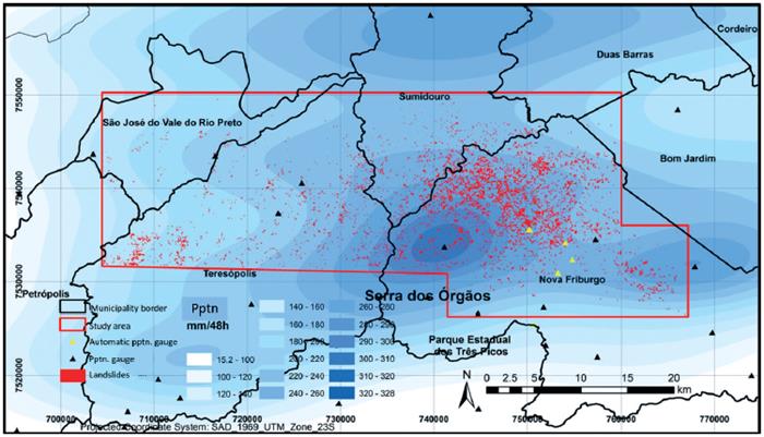
Figure 4 Map showing the landslide inventory of the extreme rainfall event on November 11-12, 2011 in "Serrana Region", Rio de Janeiro, Brazil. (Entralgo, 2013).
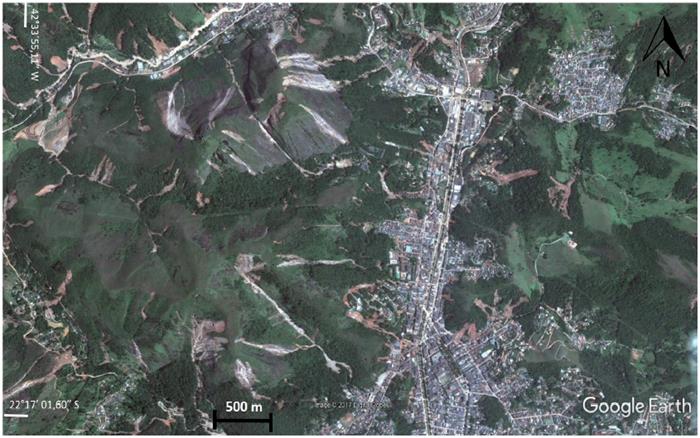
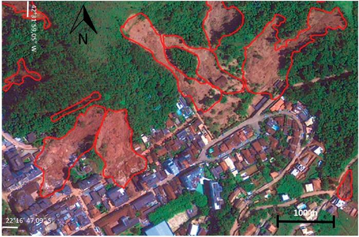
Figure 6 Typical appearance of landslides in the urban area of Nova Friburgo and effects on buildings. Graphical scale in figure.
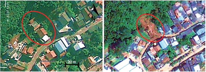
Figure 7 Comparison (before/after) of Google images that show damage to the building produced by the landslide.
Using the GIS tools, it was possible to identify the position of the buildings before landslide occurrence, as seen in Figure 8.
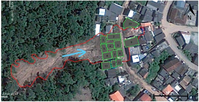
A total of 166 structures were identified, and a database was created to store landslide information (Table 1) and building information (Table 2 ).
Table 1 Example of the database for the landslide 4479.
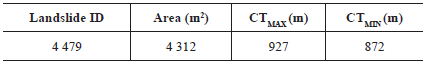
Notes: ID - Identification Number of landslide; CTMAX - Maximum height above the sea level; CTMIN - Minimum height above the sea level.
Table 2 Example of the database for the buildings affected by the landslide 4479.
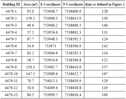
Notes: ID -Identification Number of the building; d - track distance of debris from the highest point of the landslide to the center of the building.
With the purpose of evaluating the resistance parameters for damaged buildings, according to Li´s model (Eq. 7), the Google Street View tool was used, which allows for the observation of buildings from the ground, as shown in Figure 9 and Figure 10. The observed vulnerability was initially defined in a qualitative way by discerning the degree of damage on a scale of: total (Vobs=1), intense (Vobs=0.7-0.9), medium (Vobs=0.4-0.6), and slight (Vobs<0.3).
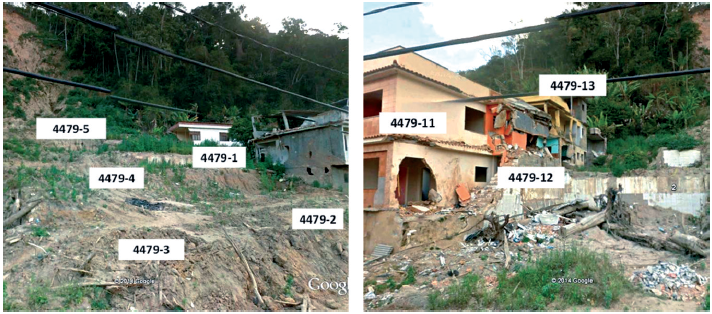
Figure 9 Floor view of buildings 1, 3, 4, 5, 11, 12 and 13 damaged by the landslide 4 479, acquired using Google Street View.
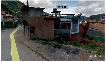
Figure 10 Floor view of the building 10 that was damaged by the landslide 4 479, acquired using Google Street View.
Resistance parameters from Li's model were properly identified, and a database was created, as shown in Table 3.
Table 3 Example of the database for the buildings damaged by the landslide 4 479.
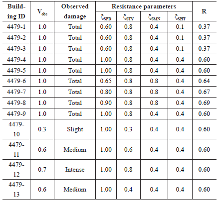
Notes: ID - Identification Number of the Building; Vobs - Observed vulnerability according to image analysis; ξSFD; ξSTY; ξSMN and ξSHT - Resistance factors accord ing to Li´s model; R - Building resistance according to Equation 7
Determination of parameters T1 and 5.
The structures that have values of observed vulnerability between 0.4 and 0.6 (medium damage) were separated from the original database, and variables Z and T were calculated. In total, only 17 structures satisfied this condition, and their calculations are presented in Table 4.
Table 4 Values of the variable T for the structures with observed vulnerability between 0.4 and 0.6.
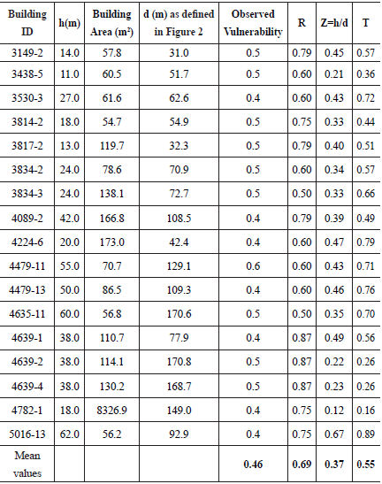
Notes: ID - Identification number of the building; h - height difference between the landslide initiation point and structure; d - track distance of debris from the highest point of landslide to the center of the building; R - Building resistance (Eq. 7); Z - modified gradient (Eq. 6); T - T-Model's main variable (Eq. 5).
The adopted strategy to calibrate the model was to use a characteristic value of the vulnerability equal to 0.5. Because the buildings affected by the Nova Friburgo landslide events presented a wide range of vulnerabilities and taking into consideration that estimation of the damage was made by direct field observation, it was decided to use those buildings that presented observed vulnerabilities in the range 0.4 to 0.6 with the purpose of having a mean value as close as possible to 0.5.
As previously mentioned in the formulation of Equation 19, the known point (T 1 ,Z 1) must be found from field observation in such a way that T1 is the “characteristic value” of T when V=V1=0.5. ´
As seen in Table 4, the mean value of observed vulnerability is 0.46. Thus, it can be approximated to 0.5. On the other hand, the mean value of variable T is 0.55. Thus, it is possible to conclude that those values precisely match the known point (T 1 ,Z 1), which has been previously defined as the "characteristic values" of the T-model.
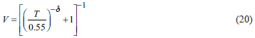
The introduction of "characteristic values" in Eq. 19, is the way to obtain Eq. 20, which is straightforward.
The next step is the calibration of the coefficient δ, which governs, on average, the relationship between the variables V and T. In the authors' opinion, δ depends mainly on the type of mass movement: debris or landslide, as shown in Figure 1. Thus, the value must be unique for all landslides that are studied in Nova Friburgo. By testing different values of δ, theoretical curves of V vs. Z were compared with the observed values. The best fit for the complete set of structures in the database was reached for δ=3.5. Thus, Equation 20 becomes
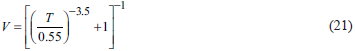
To improve visualization, Figure 11 shows the curves V vs. Z for three theoretical values of structural resistance (R=0.2; 0.5 and 0.8). The points represent observed values for all structures in the database, which are grouped into three categories: low resistance (R<0.4) - represented by an R=0.2 theoretical curve; medium resistance (0.4<=R<0.7) - represented by an R=0.5 theoretical curve; and high resistance (R>=0.7) - represented by an R=0.8 theoretical curve.
Effect of the Modified gradient (Z)
Landslides
As previously mentioned, the modified gradient (Eq. 6) is directly proportional to the height difference between the hazard location and the building and inversely proportional to the distance measured along the possible track of the sliding mass. In a qualitative sense, Z may be intended as a measure of landslide potential intensity when interacting with the structure.
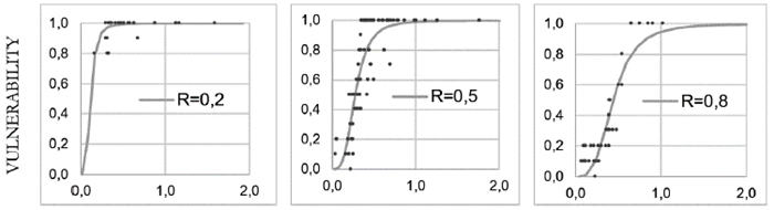
The histogram of Z (Figure 12) was prepared with all values measured in the Nova Friburgo massive landslide event, and it indicates that 70% of the cases are included in the interval (0.15<Z<0.55). In a complementary way, a histogram for the resistance was prepared, and it is presented in Figure 12. A summary of main statistics is presented in Table 5.
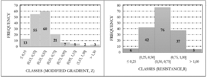
Figure 12 Frequency histogram for the modified gradient Z (left) and structural resistance R (right).
Considering the mean values of the variables involved and their standard deviations, curves of vulnerability as a function of structural resistance were prepared for three different values of the modified gradient: Zmean=0 5; Zmean+istd.dev. =0.8; and Zmean-istd.dev =0.2. These curves are presented in Figure 13 together with a schematic representation of the effect of Z in a structure with a definite structural resistance.
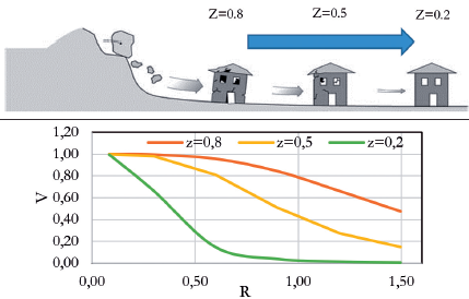
Figure 13 Effect of Z in the landslide vulnerability of buildings and curves V vs. R (structural resistance) on different values of Z. The schematic representation was adapted from Glade, Anderson, and Crozier, 2005.
Theoretical curves presented in Figure 13 show that for a specific value of resistance, the higher the modified gradient is, the higher the vulnerability. On the other hand, it is clearly shown that for low values of the modified gradient (see the Z=0.2 curve), the vulnerability significantly decreases when resistance increases. This observation may be of remarkable importance in risk management planning processes when reinforcement of existing structures is considered as an acceptable measure for risk reduction and control.
Flows
When compared to landslides, the flow-type movements are characterized by bigger sizes and long travel distances. Therefore, their interaction with buildings must be fundamentally different and characterized using a different 5 coefficient in Equation 20. To find a proper value for 5 and considering the lack of available quantitative information about damages produced by these type of processes, field observations were used, which were made in the district of "Bento Rodrigues", Minas Gerais, Brazil, which was destroyed by an earth flow that was produced by the failure of a tailings dam in November of 2015 (Figure 14)1.
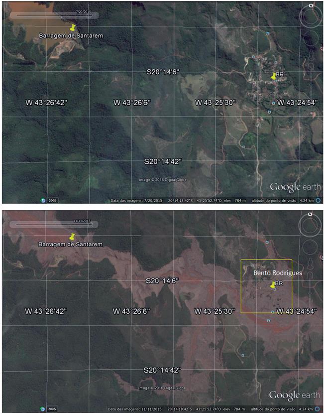
Figure 14 Aerial view (from Google Earth) before and after the failure of the tailings dam in Bento Rodrigues, Minas Gerais, Brazil. Zoomed rectangle can be seen in Figure 15.
Figure 15 shows a zoomed area where field observations were carried out three months after the tragedy. Five points were selected for the assessment of the vulnerability, as indicated in the same figure. Selected points (letters A to E) are also illustrated in the photographs of Figure 16. From the direct observation of buildings, which correspond to photos A, B and C in Figure 16, it was deduced that they presented an average vulnerability of 0.5. Thus, they can be used to calibrate the model and obtain the δ coefficient value.
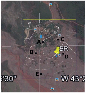
Figure 15 Detailed view of the central part of Bento Rodrigues district and five selected points for analyzing vulnerability. The values indicated on level lines correspond to the difference in height between buildings and dam breaking point.
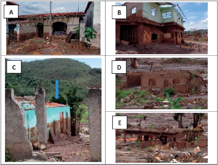
Figure 16 Photographs of selected structures located at the positions indicated in Figure 15. Photos were taken in February of 2016 during a field trip, three months after the tragedy.
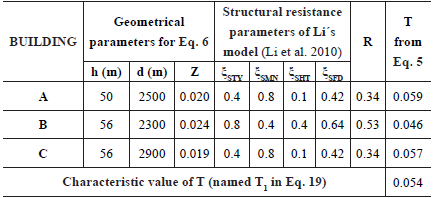
The first step is the determination of the "characteristic value" T1, which is related to V=V1=0.5. From the digital terrain model and ground GPS data, the difference in height between buildings and the dam breaking point was determined (see values on level lines in Figure 15). Table 6 presents the corresponding values. Thus, it can be concluded that T1=0.05.
Table 6 Geometrical and resistance parameters of three selected buildings with V=0.5 in Bento Rodrigues, MG, Brazil.
The next step is to test different values of δ to find the one that reproduces the observed vulnerability of all buildings. The best value is δ=1, and thus, Equation 22 is the expression used to estimate the vulnerability of buildings due to this flow-type mass movement.
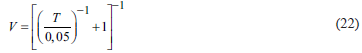
Table 7 presents the vulnerability data collected for the five selected houses in "Bento Rodrigues" and two additional structures included with the intention of verifying the consistency of the model.
Table 7 Vulnerability data for five buildings in "Bento Rodrigues", the church of "Paracatu de Baixo" district and a typical very low resistance house.
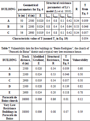
The vulnerability values of houses E and D (0.82 and 0.78 respectively) agree with the field-observed behavior (see photos in Figure 16). The additional structures are the church of "Paracatu de Baixo" district and a theoretical typical house of the region characterized, on average, as having a very low structural resistance. "Paracatu de Baixo" is a small village located approximately 38 km downstream from the tailings dam.
The village's church was partially covered by the earthflow without suffering appreciable structural damage (Figure 17).
According to newspapers, most houses of the village were destroyed. However, reliable technical information about damage quantification is not available. The estimated average vulnerability using the T-model is 0.59 (medium vulnerability), which represents significant structural damage. Considering the mean values of the variables involved, curves of vulnerability as a function of structural resistance were prepared for three different values of modified gradient Z: 0.05; 0.01 and 0.005 (see Figure 18). These curves are presented together with a schematic representation of the effect of Z in a structure with a definite structural resistance.
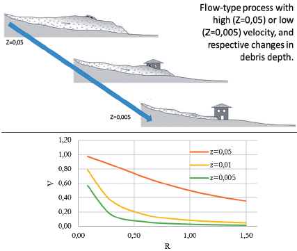
Figure 18 Effect of Z in the debris-flow vulnerability response of buildings and curves V vs. R for different values of the modified gradient, Z. The schematic representation was adapted from Glade, Anderson, and Crozier (2005).
Application of the T-Model to landslides in Medellin, Colombia
Medellin is the capital city of the Province of Antioquia, which is located in the central part of the NW Colombian Andes. The city occupies the bottom and partially hillslopes of a deep valley that is locally named the "Aburra Valley" with an extension of 1152 km2.
Due to the complex geomorphological and geological framework of the valley, several catastrophic landslides have occurred in the last century. The uncontrolled occupation of the hillslopes without adequate building practices produces a high vulnerability condition, and consequently, a very high number of lives have been claimed by massive landslides, which has also resulted in considerable economic losses (Aristizábal et al., 2011).
Figure 19 presents an inventory of the most catastrophic landslides registered in the Aburrá Valley since 1920. The last three events (La Gabriela, Poblado-Alto Verde, and El Socorro) where chosen for creating vulnerability estimations according to the T-model to verify the robustness of the model.
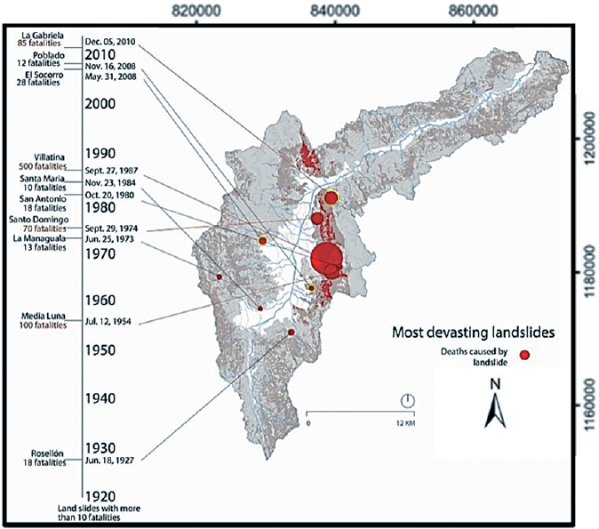
Figure 19 Catastrophic landslides in the last century in the Aburrá Valley, Colombia. Adapted from Claghorn et al. (2016).
El Socorro landslide
According to Aristizábal-Giraldo (2008), this tragic event claimed the lives of 27 people and left 16 seriously injured at the El Socorro settlement. This event, together with Rosellón (1927), Media Luna (1954), Santo Domingo (1974), Villatina (1987) and El Barro (2005), represents one of the most tragic events in the Aburrá Valley history.
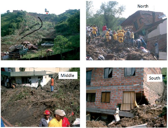
The mass movement was classified as a simple rotational landslide in the NE direction. Due to high saturation levels, the sliding mass moved 140 m ahead in the SE direction, and finally, the mass turned to the NE.
The triggering causes are associated with antecedent rainfall from the previous 15 days and a very intense rainfall event during May 30th, when 83.3 mm fell in just 2 hours and 30 minutes along the central part of the valley. In order to illustrate the reader about the precipitation regime of Medellin, it is mentioned that the mean historical precipitation for the month of May is 200 mm. Together with October (mean historical precipitation 207 mm), May is the rainiest month of the year. The driest month is January with mean historical precipitation of 52 mm. Figure 20 shows an aerial view of the landslide.
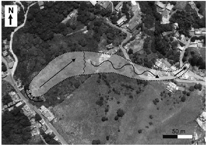
Figure 20 Aerial view of the El Socorro landslide depicting the path of the sliding mass (Aristizábal-Giraldo, 2008).
The structural resistance of the structures was determined in a generalized way from the descriptions presented in Aristizabal-Giraldo (2008) and complemented with newspaper photographs.
A total of 21 buildings were analyzed, and their vulnerability was calculated, as presented in Table 8. The location of the analyzed buildings is presented in Figure 21, where contour lines of equal Z values are shown. In comparison with the aerial view in Figure 20, it is observed that the actual path of the landslide debris is enclosed by the Z=0.3 line.
Table 8 Modified gradient (Z), structural strength (R) and physical vulnerability (V) of the buildings affected by the El Socorro landslide.
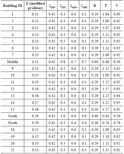
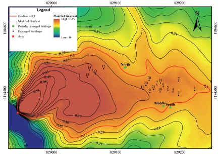
Figure 21 Location of the buildings affected by the El Socorro landslide. Points represent the buildings. Contour lines correspond to equal values of the modified gradient Z.
Because of the intensity of the landslide and the low structural strength of buildings, all houses were entirely destroyed but three, which were located at the border of contour line Z=0.3 suffered partial to intense damage only.
The mean vulnerability theoretical value of destroyed buildings is 0.92, which agrees with the catastrophic damages observed. The buildings that suffered partial damage, named north, middle and south, presented theoretica vulnerability values of 0.76, 0.39 and 0.28, respectively (Figure 22).
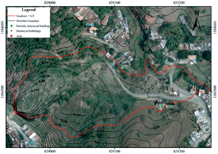
Figure 22 Location of three buildings that suffered partial damage due to the El Socorro landslide. The values indicate the vulnerability index of the buildings.
The pictures presented in Figure 23 show the level of damage sufferer by the buildings named north (V=0.8), middle (V=0.4) and south (V=0.3) The vulnerability values agree with the observed damage.
Alto Verde landslide
A massive landslide occurred at the Alto Verde residential complex at the end of 2008 in the city of Medellin, Colombia, claiming the lives of twelve people and destroying six houses (Llano-Serna, Farias, and Martínez-Carvajal, 2015). The poor geotechnical properties of Dunite residual soil and heavy antecedent rainfall were the main causes of the landslide.
Images in Figure 24 show the situation of the Alto Verde neighbourhood before and after the occurrence of the catastrophic landslide. In those images, it is possible to see the position of the six houses that were destroyed and house 1 that remained undamaged. The cross-section AA' was used by (Llano-Serna, Farias, and Martínez-Carvajal 2015) for numerical analysis of the propagation of the sliding mass using the MPM methods (Material Point Method). Detailed geotechnical information can be found in the abovementioned reference.
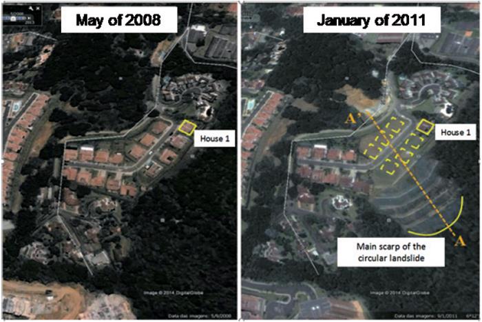
Figure 24 Aerial view of the Alto Verde landslide in 2008 (before) and in 2011 (after). House 1 remains undamaged.
The vulnerability calculations require the definition of the points that represent the position of the six destroyed houses, which can be seen in Figure 25 together with the contour lines of the modified gradient. Because of the existence of natural channels, it is necessary to limit the analysis of the modified gradient behavior to the area where the movement of the sliding mass can naturally occur. Those limits are also represented in Figure 25, which indicates that vulnerability analysis makes sense only in the area between them.
According to the literature review, the sliding mass was completely saturated, which makes the soil behave as a dense fluid. Thus, it was characterized as a debris-flow, and consequently, the parameters used in the T-model must be T1=0.05 and δ=1.
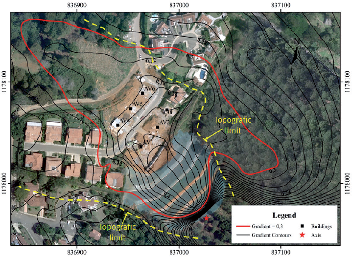
Figure 25 Location of center points representing the positions of destroyed houses during the Alto Verde landslide.
Figure 26 shows the contour map of the modified gradient (Z), which can be interpreted as a measure of the spatial evolution of the landslide intensity. As observed in the El Socorro landslide, here, the contour Z=0.3 also enclosed the limits of actual sliding mass taking into consideration the topographic limitations imposed by the axis of the natural channels mentioned before. The structures that were destroyed are numbered from AV1 to AV6, and their structural characteristics were obtained from the published literature, which is also presented in (Llano-Serna, Farias, and Martínez-Carvajal 2015).
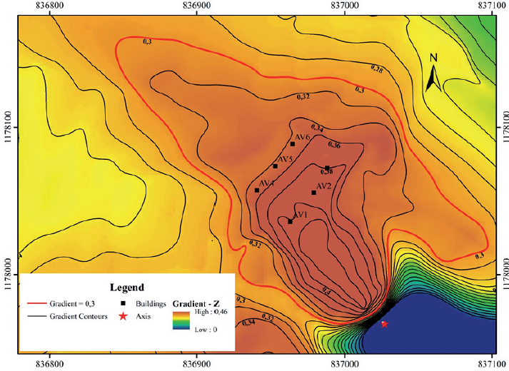
Figure 26 Contour map of the modified gradient for the Alto Verde landslide. Points AV1 to AV6 represent the position of the destroyed houses.
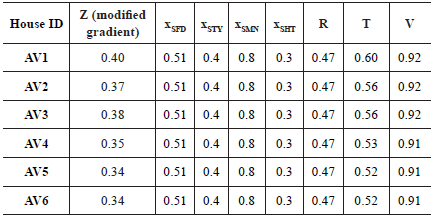
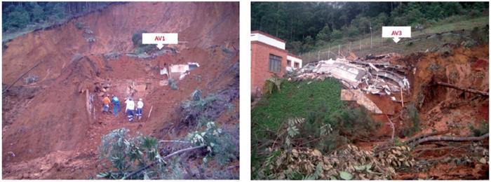
Vulnerability calculations are presented in Table 9, where the high vulnerability indexes of the houses are evident, which agrees with field observations. Despite the high structural strength of the buildings, their proximity to the sliding source and the high velocity of the sliding mass due to its flow behavior produced catastrophic vulnerability values (V>0.9). Photos in Figure 27 show the degree of destruction of houses AV1 and AV3.
Table 9 Modified gradient (Z), structural strength (R) and physical vulnerability (V) of the buildings affected by the Alto Verde landslide.
La Gabriela landslide
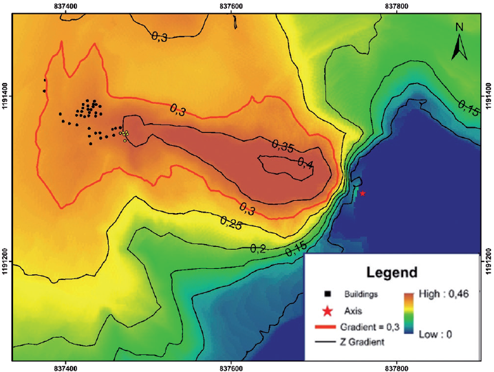
This landslide occurred on the 5th of December in 2010 during a sunny day, affected the La Gabriela neighborhood and claimed the lives of 85 people. It is unknown why a formal investigation was never carried out. Thus, technical information about the geological and geotechnical aspects is not available. The landslide main scarp was close to the Medellin - Bogotá highway in a place used by local inhabitants for placing demolition waste. Regardless of the fact that the landslide was initiated in waste material that is different from the natural soil, the decision of using the vulnerability model was justified because the theoretical background used to support the model is independent of the type of material in the sliding mass. Because the waste was not in a saturated situation, the parameters used for the T-model were T1=0.55 and 8=3.5. Figure 28 is an aerial view of the La Gabriela landslide including marks that indicate the position of damaged buildings and the topographic limit, which corresponds to a local channel that is strongly affected by gravel mining.
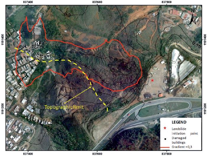
The photo presented in Figure 29 helps the reader to understand the general context of the site. The physical condition of the buildings was comparable to those described for the El Socorro landslide. In this case, 44 buildings were analyzed, and all of them had very low structural strength (Rmean=0.29).
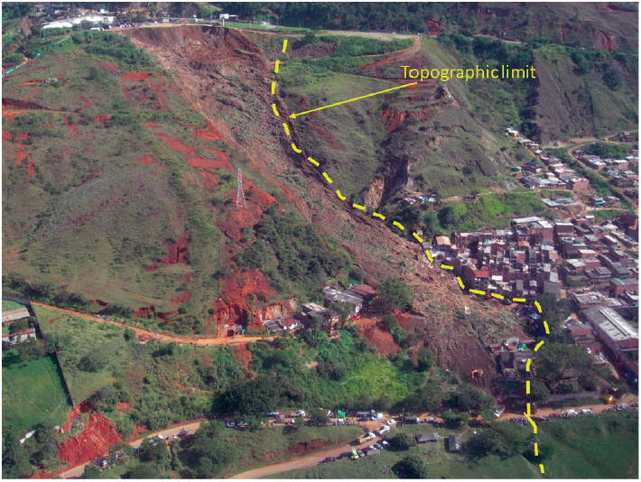
Figure 29 Panoramic view of the La Gabriela landslide. Note the topographic limit of the sliding mass.
The mean value of the modified gradient was found to be Z=0.33. Thus, the vulnerability index was 0.9 for all buildings, which agrees with the field observation of the destructiveness of the landslide.
A visual comparison between the landslide pathway and contour lines in Figure 30 allows us to conclude that the contour Z=0.3 enclosed the limits of the actual sliding mass, taking into consideration the topographic limitations imposed by the abovementioned channel.
Discussion
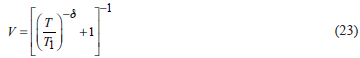
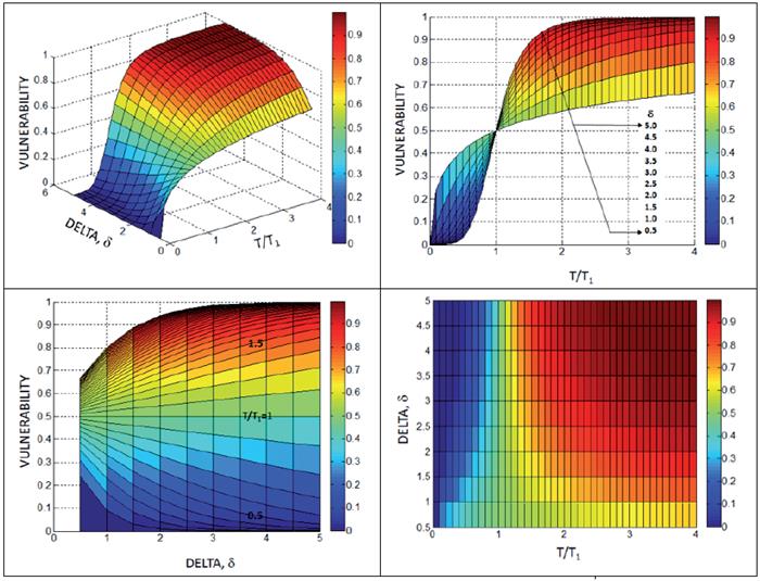
As presented before, the vulnerability model, which was explored here, is a mathematical function that depends on two main variables: T and δ (Eq. 23). The first variable takes into consideration the relationship between a measure of the potential intensity of the landslide (here named modified gradient, Z) and the structural resistance of the buildings. The coefficient δ is responsible for including the effect of different types of mass movements in the model. The characteristic value T1 must be calibrated with field observations and correspond to the value of T that produces V=0.5.
Thus, the vulnerability is a continuous surface, as presented in Figure 31, which includes all values into the real domain [0,1] depending on the combination of the type of movement and variable T.
The general expression presented in Equation 23 may be labelled universal because of its capacity for representing, in theory, the structural damage due to the interaction of any type of mass movement and any building. According to van Westen, van Asch, and Soeters (2006), the vulnerability of elements at risk, which are related to landsliding, is extremely difficult to establish for most landslide types because very limited damage data are available. Table 10 gives a schematic overview of different types of damage that may be caused by different landslide types and different elements at risk, including notes on the applicability of T-Model for assessing landslide physical vulnerability of the structures.
Table 10 Applicability of the T-Model for physical vulnerability assessment depending on the type of landslide. Modified from van Westen, van Asch, and Soeters (2006).
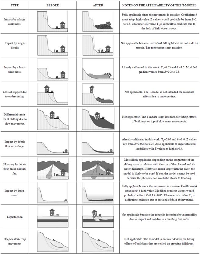
Unlike other types of hazards, such as earthquakes, flooding or windstorms, relatively little work has been done on the quantification of the physical vulnerability due to landslides (Ciurean and Schröter, 2013). The problem with landslide vulnerability assessment is that there are many types of landslides, and each one should be evaluated separately (Table 10). Such vulnerability information should come from historical studies in the first place but can be combined with modelling approaches, empirical approaches and theoretical approaches.
Assessment of the level of risk using mathematical approaches, as the T-Model demonstrated, is sufficient for use at medium to regional scales to decide which areas should be avoided for new developments or to identify areas of relatively high risk for more detailed investigation. At medium scales, the most important input data are event-based landslide inventory maps, which are made directly after any major disaster (earthquake, rainstorm, hurricane, etc.). Such an inventory by geomorphologists should emphasize landslide characteristics (types and volumes) as well as damage caused to the different elements at risk (Klose, Maurischat, and Damm, 2015).
In addition to the capability of the T-Model to represent, in theory, any type of landslide vulnerability due to the impact interaction between a mass and a building, there is a potential for easy and straightforward application in GIS environments for spatial analysis.
Conclusions
A theoretical model was presented to assess the physical vulnerability of structures that are impacted by landslides and debris flows. The vulnerability is directly proportional to the value of a new topographic variable named the "modified gradient" (Eq. 6) and inversely proportional to the structural resistance of buildings, which is measured as proposed by Li et al. (2010). The proposed theoretical model is based on a philosophical analysis of nature's behavior, which has been originally proposed in Juarez-Badillo (1985) and named the "Principle of Natural Proportionality", which establishes that all natural phenomena can be described in an ordered and simple manner using "appropriate" variables. The model was initially calibrated using the database collected from a catastrophic rainfall-triggered landslide event that occurred in Nova Friburgo, Brazil, in November of 2011. The proportionality between the variables involved in the proposed model is made using a coefficient, 8, which holds the nature of the sliding mass in a broad way, that is involving the physical characteristics of the process that governs its destructive capacity.
The results of the Nova Friburgo landslide vulnerability simulations agree with the observed damages. It was deduced that for the soil-slip landslides, such as those that occurred in Nova Friburgo, the coefficient of proportionality adopts the value of δ=3.5. In contrast, when the sliding mass behaves as a flow, the coefficient of proportionality acquires a lower value, δ=1. It was revealed that to calibrate the model, the user must look for field evidence of buildings that suffered 50% of structural damage after being impacted by landslides. Depending on the type of landslide, this damage level may appear as close as 50 m from the hazard source or as distant as a few kilometers (as in the case of low-type movements).
According to the authors' opinion, once calibrated for a certain type of mass movement, the model may be used in a general way regardless of the site or the geographical situation. Thus, the general expression for the model (Eq. 19) may be considered universal. In addition to the capability of the T-Model to represent, in theory, any type of landslide vulnerability due to the impact of an interaction between a mass and a building, there is a potential for its easy and straightforward application in GIS environments for spatial analysis, which represents one of the most important advantages over other vulnerability models that are already available. On the other hand, the introduction of the modified gradient concept and its physical interpretation leads to the direct application of the model in risk reduction processes. Values of Z=0.3 show good agreement with the actual deposition paths of the analyzed landslides.
Finally, the authors must state that the universality of the T-Model must be assumed as a simple mathematical expression. It is recognized that a real universal objective model for vulnerability to landslides is not currently practical. More important than the model itself is the methodology that is presented here to take field qualitative damage information and turn it into quantitative information in a mathematical framework.
As other vulnerability models, the T-Model is not able to fully exploit its potential until a more systematic analysis of data of the damage induced by landslides on the built environment is performed. Of course, the potential users of the T-Model must be critics in relation to the values of the parameters that are presented in this paper. The T-Model is just a modest proposal that requires further calibration and deep expert criticism.

