


 English (pdf)
 Article in xml format
 Article references
 Send this article by e-mail
 Cited by SciELO
  Cited by Google
  Similars in
SciELO
Similars in
SciELO  Similars in Google
 Permalink
Introduction
As the difficulty of finding oil and gas resources in shallow seismic exploration increases, in-depth seismic exploration is gaining more and more attention (Liang et al., 2016). However, deep seismic exploration imposes higher requirements on seismic exploration methods because of the larger area of calculation and the complexity of the structure. Seismic traveltime has a broad application in seismic exploration methods, including migration, demigration, tomography, and forward modeling (Wang et al., 2018; Sun et al., 2017; Wan, Wei & Wu, 2017; Yang & Zhu, 2017; Wang, Li & Chen, 2017; Yang et al., 2018; Huang & Sun, 2018; Wang et al., 2016; Sun et al, 2018). It is of great significance to study seismic traveltime calculation methods for in-depth seismic exploration.
Currently, traveltime calculation methods can mainly be divided into three kinds, including ray-based methods, finite difference methods, and new ray tracing methods based on graph processing techniques. Regarding ray-based methods, they can be divided into two kinds. The first kind is traditional ray tracing methods (mainly including the trial ray method and the shooting method); the second kind is Wavefront Construction (WFC). The trial ray method and the shooting method (Julian, 1977) were widely applied to seismic exploration techniques in the past, but these two methods face with prominent problems, such as low calculation efficiency and low adaptability to complex models. WFC was first put forward by Vinje (1993) and improved later by various scholars (Vinje, 1997; Coman, R., & Gajewski, 2005). Chambers and Kendall (2008) presented a practical WFC implementation method in 3D isotropic media. Hauser et al. (2008) obtained the multiarrival traveltime by the WFC method. Han et al. (2009) proposed a new positioning method for grid points in WFC. Bai et al. (2011) studied the seismic wavefront evolution of multiply reflected, transmitted, and converted phases in 2D/3D triangular cell model.
The method does not break new ground regarding principles. It is still a new technique to realize traditional ray tracing methods in essence, but the technique succeeds in playing an important role in popularizing the application of ray theories to seismic exploration. WFC boasts a good calculation precision, but its calculation efficiency is low because lots of rays are required to insert into the calculation process to ensure the ray density of the model space. Combining graph processing techniques and traveltime calculation, modern ray tracing methods mainly include: interpolation method (Asakawa & Kawanaka, 1993; Cardarelli & Cerreto, 2002; Nie & Yang, 2003); shortest ray path tracing method (Moser, 1991; Bai, Greenhalgh & Zhou, 2007; Sun Z., Sun J., & Han, 2009). These methods can help obtain both traveltime and ray paths, but their calculation process calls for the screening of authentic ray paths from numerous useless ones. Thus, methods of the kind are low in calculation efficiency.
A finite difference method for traveltime calculation was first put forward by Vidale (1988). Methods of the kind obtain the viscosity solution of the eikonal equation through numerical analysis. Their calculation efficiency is high, but their defect is striking, in that, their calculation accuracy is low especially in the area near the source. Fast Marching Method (FMM) is one of the finite difference methods, which was raised by Sethian (1996). The technique was originated from the Level Set method (Sussman, Smereka & Osher, 1994). It integrates the narrow-band technology and the heapsort technique into its calculation process to achieve high efficiency, stability, and adaptability. Due to salient advantages, FMM was favored by many scholars (Sun & Fomel, 1998; Alkhalifah & Fomel, 2001; Rawlinson & Sambridge, 2004) not long after its emergence, but it still failed to solve inadequate calculation accuracy of traveltime near the source. For the strong adaptability of FMM, it was often used for calculating models under rugged topography (Sun, Z., Sun, J. & Han, 2010; Sun, Z., Sun, J. & Han, 2011; Sun, J. & Han, 2012). Liu et al. (2014) proposed a TTI traveltime computation method based on a dynamic programming approach. Ma and Zhang (2014) obtained the ray information from the first arrival traveltime by solving the topography dependent eikonal equation. Sun et al. (2016) analyzed the effects of seawater velocity variation on deep-water seismic migration and found that the traveltime difference was a significant factor. Huang et al. (2016) solved the complex eikonal equation to obtain the traveltime by a nonuniform grid-based finite-difference method. Sun et al. (2016) traced the ray in the random media with complex topography by employing the GMM-ULTI method. Sun et al. (2017) calculated the seismic traveltime under complex conditions using the group marching upwind hybrid method. Huang and Greenhalgh (2018) further proposed an approximate solution for the seismic complex traveltime. Lan and Chen (2018) presented an upwind fast sweeping scheme for seismic traveltime calculation under the irregular free surface condition.
Based on the advantages and disadvantages of FMM and WFC, this paper puts forward a joint traveltime calculation method for deep-sea geology. According to this method, WFC is adopted for traveltime calculation in the surrounding of the source; and FMM is for the traveltime calculation of the remaining area. By improving the traveltime calculation accuracy near the source, the joint traveltime calculation method achieves the goal of enhancing the overall calculation accuracy while maintaining the high calculation efficiency of FMM. The above conclusions are verified through the error analysis of the homogeneous model and the trial of the gradient model, the layered model, the Marmousi model, and Sigsbee model.
Methods
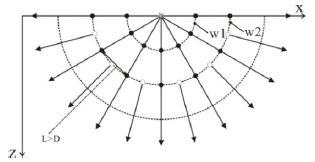
FMM is an efficient and stable method to calculate seismic traveltime. Its calculation of grid nodes' traveltime relies on the information of the surrounding nodes already derived. Since there is little node information near the source, the calculation accuracy of the area is relatively weak. Inadequate calculation accuracy in the area also influences the overall calculation accuracy. To improve the efficiency of FMM near the source is of vital importance to the improvement of the method. WFC is also an effective method for traveltime calculation. However, with the increase of the calculation area, the blind calculation zone will appear, and the calculation efficiency is not high, but its calculation accuracy near the source is relatively high. Based on the characteristics of the two traveltime calculation methods, this paper puts forward a joint traveltime calculation method based on the two calculation methods. As is shown in Figure 1, the new method employs WFC for traveltime calculation in the surrounding of the source, and FMM for traveltime calculation of the remaining area. Before introducing the joint traveltime calculation method, this part first gives a brief introduction of basic principles of FMM and WFC; then puts forward strategies to realize the combination of the two ways, and finally provides the schematic flow diagram.
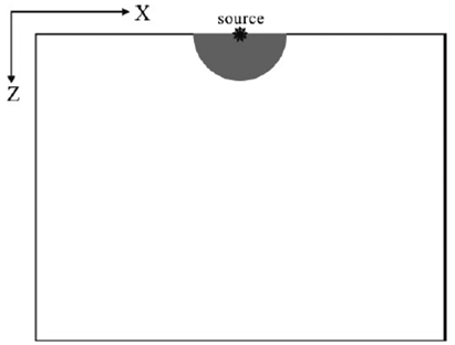
Figure 1 FMM and WFC calculation regional diagram in the joint calculation method. WFC calculates the gray region, FMM calculates the white part.
Principles of FMM
By solving the eikonal equation through the upwind method, FMM obtains the seismic traveltime. Before the introduction of the method, the 2D eikonal function is first introduced (Bai, Greenhalgh, Zhou, 2007).

Where, t is the seismic traveltime; s is the slowness; ▽ is the gradient symbol. In (1), the upwind difference of the gradient item is approximate to (Sethian, J. A., & Popovici, 1999):
Where,  and
and  are the forward and backward difference operator in the direction of x and z. Below are the specific forms:
(2) could be reduced to a simpler form:
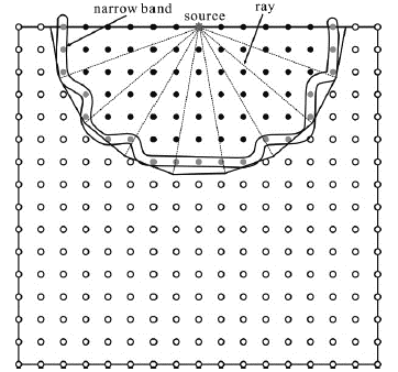
During the realization process, FMM adopts the narrow-band technique as the wavefront expansion method. The first step of the narrowband procedure is to establish the first narrow-band. Usually, the grid points near the source were selected as the elements of the first narrowband, which is shown in Figure 2. During the narrow-band initialization, traveltime of the source (i s , j s ) is zero. The traveltime of the points near the source can be expressed as
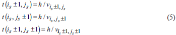
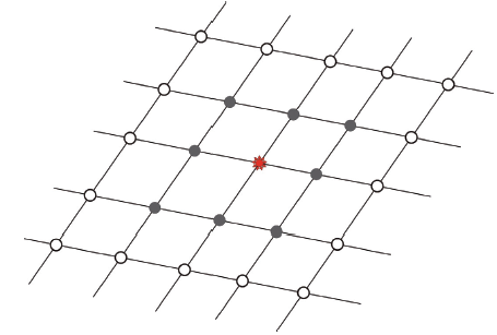
Figure 2 Narrow-band initialization. The red star is the source; gray points are the initial elements of the narrow-band.
Where, t stands traveltime; ν for velocity; h for grid space. When the traveltime calculation of the grid nodes is complete, they will be inserted to the narrow band to establish the initial narrow band.
After the narrow-band initialization is finished, the wavefront will be expanded as is shown in Figure 3. In this step, the minimum traveltime grid node within the narrow band need to be found, and the heapsort technique is employed to improve the calculation efficiency.
Principles of WFC
The theoretical basis of WFC for traveltime calculation is to solve the Kinetic Radial Tracing (KRT) equations. The KRT equations are shown below:
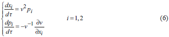
Where, x. stands coordinates in space; v for velocity; p. for slowness component product; % for the value of traveltime.
By solving the above equations, traveltime of discrete nodes along the ray paths can be obtained. For the reason that WFC is only employed near the source, just the distance factor is considered to insert a new ray to ensure the ray coverage. As is shown in Figure 4, new rays are added only when the distance is higher than the critical value.
In the joint traveltime calculation method, traveltime of regular grid nodes is needed. Below is a brief introduction of calculating traveltime of regular grid nodes based on the information along the ray paths.
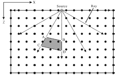
The adjacent rays and the wavefronts form irregular quadrangles. (See Fig. 5) Concerning any irregular quadrangle, ABCD, regular grid nodes within the quadrangle are first chosen out, the process of which is discussed in detail by Han et al. (2009). Then, based on the information of four Vertexes, namely A, B, C and D, the traveltime of regular grid nodes within them can be interpolated (See Fig. 6).
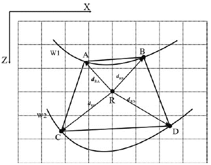
Once the position of the target point is determined, its traveltime could be calculated by the information of the quadrilateral vertices. As is the shown in Figure 7, R is the target point; A, B, C and D are the quadrilateral vertices. Oa, Ob, Oc and Od are the virtual sources, which are determined the information of quadrilateral vertices. The traveltime of R can be expressed as:
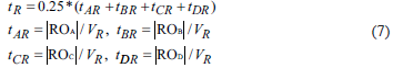
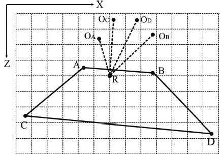
Where, V R stands the velocity at point R.
Principles and realization strategies of joint traveltime calculation based on FMM and WFC
The joint traveltime calculation method is proposed to combine the advantages of FMM and WFC. The new method calculates the grid nodes' traveltime with WFC in a small area near the source. The maximum single ray tracing distance is chosen between 5% and 10% of the model side length. Three aspects were taken into consideration when the scope was selected. Firstly, WFC takes relatively more time, so the calculation area will influence the computation efficiency of the new algorithm. Secondly, when the WFC calculation area becomes larger, it's easy to appear a blind area in the model and may need to insert new rays to satisfy the precision of the algorithm, which will further reduce the efficiency of the new method. Finally, it can be seen from the accuracy of the analysis below is that the calculation accuracy of the technique has been greatly improved when WFC is used within that scope.
Though the combination of the two traveltime calculation methods can make the best of -both in different model areas, FMM and WFC are independent of each other and have little association, so the key to realizing the joint traveltime method lies in how to combine the two ways into a whole. This process could be realized through the narrow-band technique of FMM.
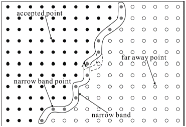
Narrow-band technique plays an essential role in FMM. As the wavefront expansion mode of FMM, it endows FMM with robust stability and flexibility. Before the use of the narrow-band technique, grid nodes in the whole space are divided into three kinds, namely accepted nodes, narrowband nodes, and far-away nodes. Accepted nodes refer to grid nodes which have been calculated and confirmed. Narrow-band nodes refer to grid nodes which have been calculated but have not yet been finally confirmed. Faraway nodes refer to grid nodes which have not been calculated. Narrowband refers to the collection of all narrow-band nodes. In FMM, it is used to stay close to the wavefront. The above process of forming the narrow band is called narrow-band initialization. In the joint traveltime calculation method based on FMM and WFC, the grid nodes' traveltime calculation sequence is: first, WFC is used to finish the traveltime calculation of the area near the source; then, FMM is used to calculate traveltime of the remaining area. Therefore, the narrow-band initialization in the joint method is a step after WFC finishing the traveltime calculation.
As is shown in Figure 8, the imaginary line stands for the length of the single ray; the nodes within the enclosed full line graph are grid nodes already calculated by WFC. As to the narrow-band initialization in the joint method, the grid nodes outside the enclosed full line graph are defined as far-away nodes. (See white nodes in Fig. 8) Nodes within the enclosed full line graph are a collection of accepted nodes and narrow-band nodes. Therefore, they should be further divided. As to grid nodes already calculated by WFC, if a grid node's surrounding (back, front, left and right) nodes are all calculated by WFC, it is defined as the accepted node (See black nodes in Fig. 8); otherwise, it is the narrow-band node (See gray nodes in Fig. 8). Move all narrow-band nodes into the narrow band to finish the step of narrow-band initialization in the joint traveltime method.
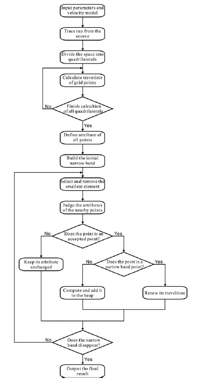
The completion of the above step means that WFC and FMM finish the connection. Below is an introduction of how to use FMM to achieve traveltime calculation of the remaining grid nodes. The process is defined as the narrow-band expansion, which can generally be divided into the following three steps: (1) Choose the minimum traveltime node in the narrow band which have been initialized through WFC, and change the attribute of the node from the narrow-band node to the accepted node; (2) Judge the characteristic of the surrounding nodes of the newly-confirmed accepted node. If the node is a far-away node, the finite difference method is employed to work out its traveltime and change its attribute to the narrowband node. If the node is a narrow-band node, its traveltime value should be updated, but its characteristic should be maintained; if the node is an accepted node, the attribute and the traveltime value of the node should both be maintained; (3) Repeat Step 1 and Step 2 until the narrow band is empty.
Through the above analysis, it can be seen that the key to the joint traveltime calculation method lies in the flexible application of the narrowband technique. The technique is a bridge to connect FMM and WFC.
Below is a realization flow diagram of the joint traveltime calculation method put forward in this paper (See Fig. 9)
EXPERIMENTS AND ANALYSIS
This part uses the homogeneous model to analyze the accuracy of the joint traveltime calculation method based on FMM and WFC, and multiple complex numerical models to verify the stability and adaptability of the new approach.
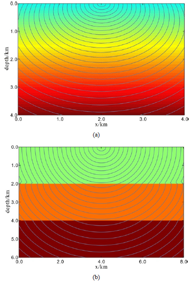
The size of the homogeneous model is 601x601; the grid spacing is 10mx10m; the velocity is 1,000m/s. In the joint traveltime calculation method, the maximum length of the single ray is 500m. Figures 10a, 10b and 10c show the relative error of the first-order FMM, the second-order FMM, and the FMM and WFC joint traveltime calculation method on the model. (The FMM used in the joint traveltime calculation method is the first order.) It can be seen that the calculation accuracy of the FMM and WFC joint traveltime calculation method has greatly improved compared with the first-order FMM, and is even higher than that of the second-order FMM.
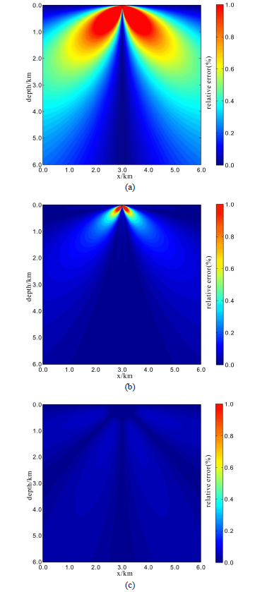
Figure 10 Homogeneous medium relative error schematic diagram: first-order FMM relative error (a); second-order FMM relative error (b); FMM and WFC joint traveltime calculation method relative error (c).
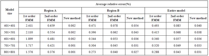
Table 1 shows the calculation accuracy of the joint traveltime calculation method put forward in this paper in different areas. The traveltime calculated by the joint method can be divided into two parts: one part is traveltime obtained through WFC, and the collection of the regular grid nodes in the area is called A; the other part is traveltime obtained through FMM, and the group of nodes of this part is called B. Table 1 shows that the average relative error of the three methods in Part A, Part B, and all grid nodes. Regarding velocity models of different sizes, the ratio of the maximum ray tracing length to the model's unilateral length is 1:12. In this way, the number of grid nodes in Part A steadily accounts for around 1.1% of the total. From Table 1, it can be seen that the accuracy of the joint traveltime calculation method based on the first-order FMM and WFC registers an obvious improvement compared with the first-order FMM. The joint way improves the calculation accuracy not only in the area of Part A through WFC, but also in the area of Part B. Though Part B is calculated through the first-order FMM, it can be seen that, due to the improvement of the traveltime calculation accuracy in Part A, the calculation accuracy of the first-order FMM in Part B is higher than that of the second-order FMM.
Table 1 The average relative error comparison between Fast Marching Methods and the method combining the Fast Marching Method with the Wavefront Construction Method.
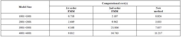
In the former part, the calculation of the joint traveltime calculation method is analyzed. The following section is an analysis of the new method's calculation efficiency. Table 2 shows the time consumed by the calculation of homogenous models of different sizes through the first-order FMM, the second-order FMM, and the joint traveltime calculation method. It can be found the calculation efficiency of the new approach is a little lower than that of the first-order FMM but is far higher than that of the second-order FMM. Generally speaking, the FMM and WFC joint traveltime method has good accuracy and efficiency.
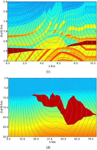
Complex models are adapted to verify the stability and adaptability of the FMM and WFC joint traveltime calculation method. Figure 11a is the isochronal graph of the gradient model, whose model size is 401 x 401; the grid spacing is 10m x 10m ; the velocity distribution is v = 1000m + 0.4z. Figure 11b is a layered medium, whose model size is 801 x 601; grid spacing is 10m x 10m; the up-down layer velocity is 1500m/s, 2000m/s and 2500m/s, respectively. Figure 11c is the isochronal graph of Marmousi model, whose model size is 2085 x 603; grid spacing is 5m x 5m. Figure 11d is the isochronal graph of Sigsbee model, whose model size is 3210 x 1201; grid spacing is 25m x 25m.
Based on the calculation results of Figure 11, it can be found that the new method can obtain the traveltime results met the laws of seismic wave propagation and boast good stability and adaptability to complex models.
Conclusions
FMM boasts high stability and efficiency while calculating the seismic traveltime, but the calculation accuracy near the source is low, which might influence the accuracy of the whole calculation method. In response to the problem, this paper puts forward a joint traveltime calculation method based on FMM and WFC. The core idea of the new way is to calculate the small area near the source with WFC and calculate the major remaining area with FMM. The calculation accuracy and calculation efficiency of the joint calculation method are analyzed, and the complex geological models are adapted to verify that the joint traveltime calculation method put forward in this paper is a seismic traveltime calculation method accommodating to both calculation efficiency and accuracy and boasting strong stability and adaptability. The new approach can serve as a powerful traveltime calculation tool for seismic exploration techniques, such as migration, demigration, and tomography.

