


 Inglês (pdf)
 Artigo em XML
 Referências do artigo
 Enviar este artigo por email
 Citado por SciELO
  Citado por Google
  Similares em
SciELO
Similares em
SciELO  Similares em Google
 Permalink
Introduction
The increasing mobility of people and goods, as well as the rapid growth of users of mobile devices with location-based services, significantly expands the need for geospatial information gathered from artificial Earth satellites. To address this challenge, the integrity of the multi-GNSS (US American GPS, Russian GLONASS, European Galileo, and Chinese BeiDou) propagated into national or international positioning services is of great importance. The GPS (Global Positioning System) can be highlighted here due to the stability of the system over a long period of time and the robustness of its signals. Initially, its satellites emitted the signals in two frequencies (L1 and L2) only. Over the years, on the basis of its modernization program, the outdated satellites of the space segment of the GPS were replenished by satellites of new generations emissions as well new navigation signals that were added to the existing signals (Leick, Rapoport, and Tatarnikov, 2015; Segantine, 2005). However, one of the advantages of dual or triple-frequency receivers is the possibility of making linear combinations between the observables of different carriers to improve the positioning accuracy by reducing the ionospheric effect and by also eliminating the errors of receiver and satellite clocks.
In recent years, to avoid the high costs associated with the use of double or multifrequency receivers, some studies have been conducted to assess the possibility of using superficial artificial neural networks (ANNs) to generate L2 carrier observations from data gathered by a single-frequency receiver within a continuous monitoring network (Mazzetto, 2017; C. A. U. da Silva, 2003). Although some unsatisfactory results were obtained in certain tests during the learning process of the networks, in general, the relative positioning solutions estimated using the generated L2 observables were more accurate than those using the original L1 data only. This suggests that it is possible to model the behavior of GPS observations for up to 30 minutes to generate the L2 carrier observables, improving the positioning accuracy of low-cost single-frequency receivers.
According to Hornik, Stinchcombe and White (1989), a shallow Multilayer Perceptron (MLP) can approximate any function at a particular accuracy level. However, Bengio and Lecun (2007) argue that although networks with one hidden layer have advantages, deeper models can represent some systems more efficiently because they can learn lower-level abstractions (characteristics of the characteristics). In addition, Goodfellow, Bengio and Courville (2016) have shown from empirical tests that ANNs with two or more hidden layers have a better generalization capacity than the simpler models. Thus, this paper aims to implement ANNs with more than one hidden layer, through the TensorFlow library in the Python computer language, to estimate the GPS L2 carrier observables. In addition, the present investigation seeks to validate a network topology through the cross-validation (CV) technique by random sampling and compare the results with those obtained in other research.
Literature Review
This research requires the union of two areas of knowledge: Geodesy, with a GPS problem in geomatics, and computer science, with ANNs being a possible solution. Due to this association, it became necessary to detail the state of the art of ANNs and their applications in the area of geomatics and similar areas.
Starting with the ANN theme, Mcculloch and Pitts (1943) developed the concept of the first artificial model of a biological neuron, exhibiting its computational capacities. Posteriorly, Rosenblatt (1958) proposed a new model named Perceptron. In the following years, Widrow and Hoff (1960) created the Delta learning rule to minimize the errors of an ANN based on gradient descent. In 1982, Hopfield's proposition of a recurrent ANN gave the area quite prominence, and in the following years, the backpropagation algorithm creation (Rumelhart, Hinton, and Williams, 1986) and computational advances have consecrated the ANN studies.
Several practical applications have since been performed with ANNs. Among the research developed, there is a current that relates them to the satellite positioning segment with the GNSS. In Mosavi (2004), ANNs were used in the estimation of observations corrections for Differential Global Positioning System (DGPS). Furthermore, Kubik and Zhang (1997) and Indriyatmoko et al. (2008) also applied the ANN tool to predict the DGPS corrections.
Jwo and Chin (2002) used a superficial ANN to determine the Precision Geometric Dilution (GDOP) parameter, and Jwo and Lai (2007) conducted tests with several architectures and topologies, trying to select the ideal configuration to estimate GDOP values. The results showed that all candidate networks met expectations regarding the accuracy of their outputs, but those trained by the backpropagation algorithm presented a longer learning process. In addition, a Recurrent Wavelet Neural Network (RWNN) was implemented in Mosavi (2007) to reduce GPS receiver time data noise and to model the errors of this source.
ANNs were also applied to improve positioning during GPS signal blocking. Semeniuk and Noureldin (2006), for instance, created an alternative method based on an ANN that estimates the speed and position errors of an inertial navigation system to correct and improve positioning in locations where the GPS system is not available. More recently, a hybrid between a Wavelet Neural Network (WNN) and the Strong Tracking Kalman-Filter (STKF) was proposed in an attempt to improve the positioning by satellites during this type of situation (Chen et al., 2013). The combination of these two tools in the work of Chen et al. (2013) was based on the WNN outstanding performance in data prediction and on the capacity of the STKF to estimate Inertial Navigation System (INS) errors. Thus, it has been proposed to represent a sequential process because when there is no blockage in the GPS signal, the WNN is trained using the predicted prior positioning errors, which were provided by the STKF, and it generates, as an output, the current positioning error.
Approaching the topic of this paper, Silva (2003) sought to improve the positioning with single-frequency receivers, creating a method to estimate the GPS L2 carrier observables using an ANN. For estimating the L2 carrier phase, an MLP with one hidden layer and 6 artificial neurons was chosen; for estimating the L2 carrier code, the author adopted the same architecture but with 30 artificial neurons in one hidden layer. Both configurations were implemented in MATLAB 6.1 and trained by the Levenberg-Marquardt algorithm, reaching up to 5,000 iterations. The results of Silva (2003) indicate that the tool can successfully model the observable behavior.
In another investigation, Leandro, Silva and Santos (2007) evaluated the best method for feeding an ANN with GPS observations. In addition, Mazzetto (2017), adopting the same topologies indicated by Silva (2003), proposed a method in which only the signals with higher strength obtained in four stations near the receiver, where it is desired to estimate the observables, should be used because, theoretically, they experience the same atmospheric effects. In this research, ANN training processes required up to 8 minutes and 15,000 iterations to complete. Although so much time has been expended, some validation MSE values were quite high and not converging as expected. Despite these factors, he was able to increase the prediction time of the GPS observables and improve the positioning accuracy in certain tests performed.
The literature review showed that the studies used only an intermediate layer ANN to estimate the GPS L2 carrier observables. In addition, there is no ANN topology validated through the CV technique to estimate the GPS L2 carrier observables. Therefore, the use of an appropriate ANN model to estimate the L2 carrier data, capable of extracting the characteristics of the process more eficiently than a shallow MLP and being tolerant to the noises present in the input signals, represents an important step towards the enhancement of postprocessed solutions with single-frequency devices.
Materials and Methods
In this investigation, it was decided to implement the network in the TensorFlow library through the Python language. Designed initially for machine learning applications, the low-level structure tool is currently being used in different fields and by several large companies (TensorFlow, 2018).
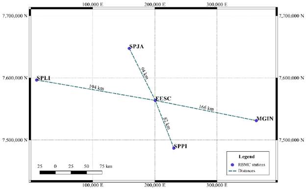
To select the appropriate ANN model, the CV technique was applied, bypassing the training and validation samples, which were obtained in the dual-frequency RINEX files generated in the Inconfidentes/MG (MGIN), Piracicaba/SP (SPPI), Lins/SP (SPLI) and Jaboticabal/SP (SPJA) stations. Then, the ANN was tested in the L1 carrier observables generated in the receiver fixed in São Carlos/SP (EESC). Figure 1 shows this configuration, chosen to compare the results obtained with those obtained in previous works, to evaluate the performance of the new model using exactly the same data used by Mazzetto (2017).
Next, Table 1 shows the test dates and times.
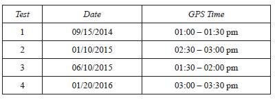
The variation in the ionospheric refraction mainly depends on the latitude of the station, the angle of elevation, and the time of observation. Near the magnetic equator, the ionospheric refraction varies more rapidly in time. Hence, in our example, we use data of satellites that were received on different days between 01:00 and 03:30 pm due to strong solar activities.
The MSE values were calculated according to Equation 1.

where:
N: number of samples;
d i : observed output i (true value);
y i : predicted output i.
It is important to highlight that this proposed method for generating the L2 carrier observables was applied after the L1 carrier data were collected; that is, the estimation of these values was not performed in real-time with the ANN in the receiver. In addition, the positioning solutions originated based on data postprocessing.
For the extraction of the GPS observables from the RBMC station RINEX iles, the RINEX ADAPTER software was used. This program was developed in the research of Mazzetto (2017). In the creation of new RINEX files with the artiicial observables, the software deletes the original L2 carrier data and multiplies the L1 carrier phase values in the irst epoch (from each satellite) by a factor k, or any other desired value, to determine the initial number of the L2 carrier phase since the ambiguity term is unknown.
The generation of observations occurred differently for each type of observable, as these do not behave equally over time. Thus, two ANN models were implemented: one that used the phase differences of the L1 carrier as the input signal and the phase differences of the L2 carrier as the output. The second model used the C/A code observations as input signal and the P2 code data as the output, using the reverse truncation process. A similar method for treating observable GPS for ANNs was used in Leandro, Silva and Santos (2007).
The topology for each ANN, that is, the optimal number of hidden layers and neurons, the optimization algorithm and other parameters, was determined with tests that used the random subsampling cross-validation technique, where the available dataset was randomly subdivided into training and validation subsets five times (CV = 5), seeking to analyze the performance of each candidate towards data drawn differently for each test (Haykin, 2008; I. N. Silva, Spatti, and Flauzino, 2010).
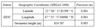
The new RINEX iles produced with the artiicial observables were processed in Geo Ofice software v. 5, from Leica, available at the Department of Transportation Engineering, at São Carlos School of Engineering (University of São Paulo), by the relative method to the EESC station with the other four stations as references. The positioning solutions were evaluated for the accuracy of the coordinates and compared with those produced by previous research. Table 2 shows the oficial coordinates of the EESC RBMC station used to determine the accuracy of the positioning solutions.
The basic processing settings adopted in the Geo Ofice 5.0 software were L1 and L1 + L2 frequencies; Hopfield tropospheric model; Leica Geo Office Standard (Standard) v. 5 ionospheric model; broadcast ephemeris; elevation mask: 15°; and GPS system data only.
The GNSS device models used in this work are the following:
1) EESC à receiver: Leica GR10; antenna: Leica AR10 (773758);
2) SPJA à receiver: Trimble NETR8; antenna: GNSS choke ring (TRM59800.00);
3) SPLI à receiver: Trimble NETR8; antenna: GNSS choke ring (TRM59800.00);
4) SPPI à receiver: Trimble NETR8; antenna: GNSS choke ring (TRM59800.00);
5) MGIN à receiver: Trimble NETR5; antenna: zephyr GNSS geodetic model 2 (TRM55971.00).
The spatial deviations (SD) were calculated according to Equation 2.
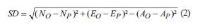
where
N 0 = the official North coordinate, in meters;
E 0 = the official East coordinate, in meters;
A0= the official Geometric altitude coordinate, in meters;
N p = the processed North coordinate, in meters (relative positioning method);
E p = the processed East coordinate, in meters (relative positioning method).
A p = the processed Geometric height coordinate, in meters (relative positioning method).
Results and Discussions
In this section, we first present the tests and results regarding the choice of the topologies of each ANN model, validated by the CV technique by random sampling. Then, the training times and the validation MSE of each test are shown. Finally, the spatial deviations of each positioning solution using the artiicial observations were compared with those obtained in other works and with the single-frequency iles.
ANN Implementation
The initial step was to develop the generic algorithm of a network, from the input data loading and normalization to the determination of the number of hidden layers, neurons and mathematical models. It is known that the optimal topology selection of an ANN occurs through attempts and errors. Each problem requires a different model. With the generic MLP, the tests were started with the observations obtained in the SPJA, SPLI, SPPI and MGIN RBMC stations.
The evaluation of the best model was due to the search for lower validation MSE values in the four experiments.
Carrier Code ANN Model
First, the intervals in which the data should be normalized was tested, choosing the limits between 0 and 1. This step was performed through the class MinMaxScaler, provided by the package Scikit-learn (Scikit-learn, 2018). The restriction of the network inputs in relation to signal strength (0, 5 and 7), as successfully proposed in Mazzetto (2017), was applied in the present investigation. However, inserting all the observations of the code without eliminating those of lower quality proved to be the best option, unlike his conclusion. This situation can be explained by the noise tolerance in the input signals that the newly implemented ANN has developed.
Regarding the number of hidden layers and the number of neurons, several topologies were investigated. Figure 2 shows the average validation MSE values for each tested configuration. Although the results are from one date, the other learning processes and the results obtained on other days were similar to those shown in the image below.
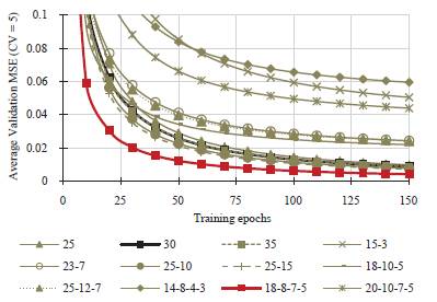
Figure 2 Comparison between models with different numbers of hidden layers and artificial neurons - Day 01/20/2016 - Fourth test day (03:00 - 03:30 pm)
In black (30), the topology chosen in Silva (2003), applied in Mazzetto (2017), and in red (18-8-7-5), the configuration chosen in this investigation are shown.
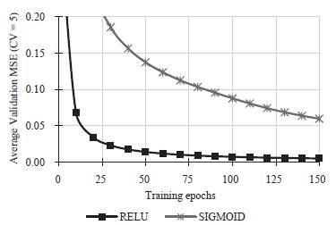
In relation to the tests performed to choose the activation function, Figure 3 shows a test that analyzed the rectified linear unit (ReLU) and logistics (SIGMOID) functions. It is observed that the ReLU produced lower validation MSE values, although in some evaluations, both functions performed satisfactorily, but with ReLU converging faster. Geron (2017) states that in practice, this function generally produces excellent outputs, is fast in processing, and works well in deep networks.
To select the optimization algorithms available in the TensorFlow library, only the two most popular algorithms were used: Adam and the stochastic gradient descent (SGD). Based on Figure 4 (MSE values reached for 09/15/2014), it is possible to verify that the former presented higher efficiency, converging rapidly. This result was expected because Kingma and Ba (2014) already demonstrated the effectiveness of the algorithm in training MLPs, comparing it with four others.
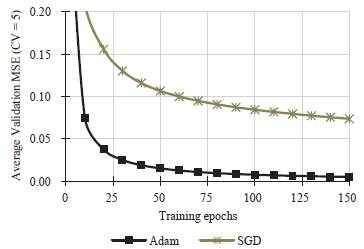
Figure 4 Comparison between optimization algorithms - 09/15/2014 - First test day (01:00 - 01:30 pm)
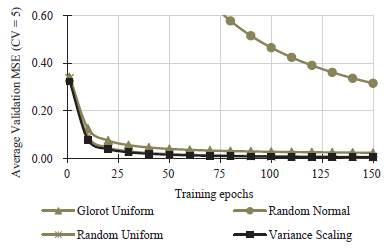
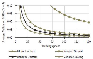
The method for initializing the synaptic weights in each layer was also tested by choosing the variance scaling type, whose objective is to keep constant the variance scale of the input signals to the final layer of the network. Figure 5 presents the average validation MSE values for tests performed on 06/10/2015.
Carrier Phase ANN Model
For the carrier phase, again using the MinMaxScaler class from the Scikit-learn library (Scikit-learn, 2018), the data were normalized between the intervals -1 and 1, reducing the propagation of the error, as the normalization factor is smaller (Leandro et al., 2007). In addition, at this stage of the research, it was chosen to restrict signal strength (intensity equal to 5), training the ANN only with the highest quality observations.
The tests on the number of hidden layers and neurons were limited to evaluating only one or two intermediate layer topologies since, above that, overfitting of the samples was verified. Figure 6 shows the results obtained for the fourth test day (01/20/2016). In red (8), the topology selected in this work is highlighted, and in black (6), the configuration adopted by Silva (2003) and used in Mazzetto (2017) is shown.
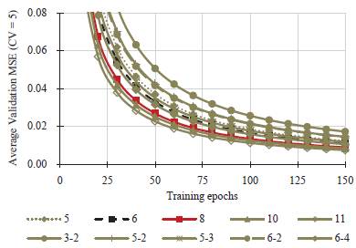
Figure 6 Comparison between models with different numbers of hidden layers and artificial neurons - Day 01/20/2016 - Fourth test day (03:00 - 03:30 pm)
Regarding the activation functions, two types were investigated: linear and hyperbolic tangent (TanH). Figure 7 shows the results.
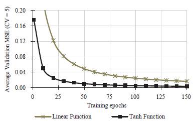
Based on all tests, it was found that the TanH function converged faster and produced the best positioning solutions and, for these reasons, was adopted for the ANN of the carrier phase.
Regarding the optimization algorithms, Adam and SGD were tested again, and the first algorithm was chosen because it provided the best results. Figure 8 shows one of the tests carried out that corroborates this conclusion.
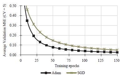
Figure 8 Comparison between optimization algorithms - 06/10/2015 -Third test day (01:30 - 02:00 pm).
Finally, the last analysis verified which initialization methods of the synaptic weights generate the lowest validation MSE values. According to Figure 9, it is observed that starting weights randomly and with a uniform distribution generated good results.
ANN Training and Validation
With the network configurations and all parameters selected, the L2 carrier phase and code observations of the EESC station were generated for the four days. Table 3 shows the total sum of training epochs of the ANNs, the learning time and the validation MSE for each observable..
Table 3 Total sum of the number of training epochs and time for generating the L2 carrier observables
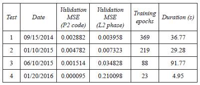
It was verified that the MSE performance parameter of the code presented very low values, close to zero, unlike the ones exposed in previous works (Mazzetto, 2017), where these numbers were not even below the unit. In general, the number of training periods of ANNs, considering both models, represents only 1.9% of the number of iterations that were performed in past research for the same sample data, while the total process time equals only 8.1%. These numbers point to the optimization of the process of generating observations with ANNs, being considerably faster, even when adopting models with more than one hidden layer.
GPS Data Processing
As the main objective of this paper was to evaluate the possibility of improving positioning solutions using ANNs, this section shows the results regarding the processing of GPS data with artificial observables. Parallels were made between the deviations obtained with the single-frequency solutions; the L1 + L2modif data, obtained in Mazzetto (2017); and the L1 + L2a observables generated in the present investigation, aiming to prove the validity of the proposed method.
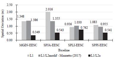
Figure 10 shows the spatial deviations (SD) obtained in processing for the first test day.
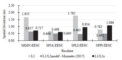
For the second test (01/10/2015), spatial deviations are shown in Figure 11. Next, Figure 12 shows the spatial deviations obtained on 06/10/2015 (Test 3).
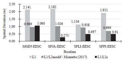
Finally, the spatial deviations of the processing performed on 01/20/2016 (Test 4) are shown in Figure 13.
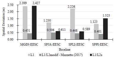
As the above figures demonstrated, applying the L1 carrier observations together with those of the L2 carrier, which were generated in this work, it was possible to reduce the positioning errors in several baselines (on average, a 40.2% reduction) when compared to the results obtained with only the original L1 data. Therefore, it can be stated that the process of GPS L2 carrier observables estimation using ANNs can improve relative positioning solutions with data obtained in single-frequency receivers.
Conclusion
Dual-frequency receivers help to improve the positioning accuracy by enabling the formation of linear combinations between the observables of different carriers. This allows us to use differencing techniques between the phase or code measurements in data processing to reduce the ionospheric effect and to also eliminate the errors of receiver and satellite clocks. Those so-called geodetic receivers are associated with high costs and, therefore, are waived by the service provider in many cases, especially in large-scale networks where a high number of these types of instruments are needed. In recent years, some studies have been carried out to check the achievable accuracy using the generated L2 carrier observations based on data gathered by a single-frequency receiver. This study aims to determine the quality of the GPS L2 carrier observables estimated by applying ANNs to answer the question of whether a dual-frequency receiver can be replaced by a cost-eficient single-frequency receiver approaching its achievable accuracy.
For this purpose, according to the literature review, for the first time, two ANN topologies were validated and selected through the CV technique to estimate the GPS L2 data, among a wide universe of possible configurations. Concisely, the MLPs selected in this research contain up to 4 hidden layers and 38 processing units. Despite this, the training and validation process of the models was extremely fast, only a few seconds, and represented less than 10% of the time spent in other research. Regarding the validation MSE values, all numbers were very close to zero.
It was veriied that by applying the observations estimated by the ANNs, together with the irst carrier originals, it was possible to achieve signiicant reductions of the spatial deviations in several baselines when compared to those obtained with only the L1 observable. In addition, some vectors presented smaller errors than those presented in Mazzetto (2017), and others have complied with the INCRA rural georeferencing standards, which determine a plane deviation of less than 50 cm. However, it should be noted that it was not possible to apply the L3 (iono-free) combination in the relative processing of the dual-frequency RINEX files, similar to what has been evidenced in previous research.
For future research, the use of genetic algorithms in the search for an even better ANN configuration for this problem is indicated, as they can analyze a vast number of candidates in a much shorter period of time than a human would need. Additionally, as future research, it is proposed that an analysis be performed to identify which factors influence the final results of the GPS data processing because, in some tests, the ANN could not successfully estimate the observations of the L2, resulting in positioning accuracy degradation when using the artificial observables.

