


 Inglés (pdf)
 Articulo en XML
 Referencias del artículo
 Enviar articulo por email
 Citado por SciELO
  Citado por Google
  Similares en
SciELO
Similares en
SciELO  Similares en Google
 Permalink
Introduction
2D and 3D representations in hydrological modeling allow to exemplify static and dynamic conditions of hydrogeological systems in natural or hypothetical scenarios, and their relationships with surface water bodies and atmospheric inputs (Alberti, Colombo, & Formentin, 2018; Gogu, Carabin, Hallet, Peters, & Dassargues, 2001). This type of modeling can be used to analyze the effects of groundwater extraction, to evaluate irrigation strategies in order to establish an appropriate correspondence with aquifers, or to simulate different water management scenarios (White, 2018). These models are classified in three types (Hughes, 2016; Sieber, Yates, Huber-Lee, & Purkey, 2005): i.) Physical models that follow the laws of physical and chemical processes, and can be determined and described by differential equations, ii.) Analogs, which are simulations of electrical order and iii.) Mathematics: which are simplified representations of physical processes that are expressed in mathematical terms to simulate complex processes taken from a specific key component of a determined system. However, hydrogeological modeling implies a variety of data that generally has little availability, especially in regions where geographical and climatic changes do not allow constant measurement (Comunian & Renard, 2009). This is why the calibration of hydrogeological models is important (Klaas, Imteaz, Sudiayem, Klaas, & Klaas, 2017).
The calibration process must be used to acquire reliable modeling results (Wu, Liu, Cai, Li, & Jiang, 2017). A good calibration of a model ensures that the vestigial data between the observed and the simulated data are minimized and the parameters uncertainties are lower (Gan et al., 2018; Simmons et al., 2017). This procedure was developed using the inverse method (M. Usman et al., 2018; X. Wang, Jardani, & Jourde, 2017). The inverse method application and the non-linear parameter estimation techniques are common in hydrogeological modeling (Carrera, Hidalgo, Slooten, & Vázquez-Suñé, 2010; X. Wang et al., 2017; White, Fienen, & Doherty, 2016). This given the swiftness that this technique shows to determine the best adjustment parameters, applying low subjectivity in the calibration procedure and also the availability of hydrogeological modeling software to easily integrate the hydrological results (N.-Z. Sun & Sun, 2015; M. Usman et al., 2018; Zhou, Gómez-Hernández, & Li, 2014). Despite this advantage, the method is limited to the satisfactory sampling of field data (Llopis-Albert, Merigó, & Palacios-Marqués, 2015; Pool, Carrera, Alcolea & Bocanegra, 2015; H. Zhang, Li, Saifullah, Li, & Li, 2016). Additionally, hydrogeological models have a high spatial-temporal variability rate that causes non-linearity which also increases the correspondence within different model input parameters (Gaganis & Smith, 2006; Marchant & Bloomfield, 2018). An unwanted effect in this situation can be the appearance of unrealistic parameter distributions, or the calibration falling into a local minimum without exploring other declines (Hu & Jiao, 2015; Klaas et al., 2017). Bearing in mind that the calibration process does not guarantee the total model reliability and that the results obtained are as real as the veracity in the assumptions used in the conceptual model (Betancur, Mejia, & Palacio, 2009; Kpegli, Alassane, van der Zee, Boukari, & Mama, 2018; Linde, Renard, Mukerji, & Caers, 2015), it is appropriate to analyze the sensitivity and uncertainty associated with the parameters. The uncertainty in the hydrogeological models is related to: i.) inaccurate measurement of input data, ii.) inadequate simplification of the represented system and iii.) calibration process (Carrera, Mousavi, Usunoff, Sánchez-Vila, & Galarza, 1993; Chen, Izady, Abdalla, & Amerjeed, 2018; Meeks, Moeck, Brunner, & Hunkeler, 2017). In particular, the calibration process of any hydrogeological model is based on some method of spatial characterization or zone focused parameters (B. Dewandel et al., 2012; Benoît Dewandel, Jeanpert, Ladouche, Join, & Maréchal, 2017). The model of this research was divided into different hydrogeological units based mainly on geological properties (Custodio et al., 2016; Islam et al., 2017; T. Wang et al., 2014). This subdivision leads to suppose hydraulic uniformity properties in each zone (Cherry et al., 2004). meaning that the hydraulic parameters values at any location are weighted averages of the actual values measured at different points within an area (Hassane Maina, Delay, & Ackerer, 2017; Irsa & Zhang, 2012; M. Zhang, Burbey, Nunes, & Borggaard, 2014). The sensitivity analysis allows to address uncertainties identifying the most important model input parameters (Karay & Hajnal, 2015). Additionally, this analysis provides an overall system understanding, reduces uncertainties and improves the calibration and validation processes (Carrera et al., 1993; Ehtiat, Mousavi, & Ghaheri, 2015; Sanchez-León, Leven, Haslauer, & Cirpka, 2016).
The use of those CZ for the values assignation to hydraulic parameters can lead to unnecessary uncertainties in the modeling and, therefore, to produce erroneous parameter values and current geological homogeneity (Linde, Ginsbourger, Irving, Nobile, & Doucet, 2017; Tiedeman & Green, 2013; Woodward, Wöhling, & Stenger, 2016). Having this into consideration, the PP technique has been proposed to help improve the spatial variability interpretation of parameters, in cases of groundwater flow modeling that cannot be obtained by working with CZ (Christensen & Doherty, 2008; Jiménez, Mariethoz, Brauchler, & Bayer, 2016; Le Ravalec-Dupin, 2010; M. Usman et al., 2018).
This technique interpolates the spatially correlated hydraulic properties values of a set of points distributed along the model domain (Ma & Jafarpour, 2017); generating a uniformed distribution of parameter values with less uncertainty. However, the use of a larger number of PPs or the area subdivision could result in extensive modeling times (Christensen & Doherty, 2008; White et al., 2016).
The application of this technique has been widely used throughout many related issues as shown (A. Alcolea, Carrera, & Medina, 2006, 2008; Christensen & Doherty, 2008; Hernandez, Neuman, Guadagnini, & Carrera, 2003; Jung, Ranjithan, & Mahinthakumar, 2011; Le Ravalec-Dupin, 2010; Le Ravalec & Mouche, 2012; Ma & Jafarpour, 2018; Panzeri, Guadagnini, & Riva, 2012). Nonetheless, the use of this technique can generate over-parameterization, situation that would lead to the optimization problem instability (Amini, Johnson, Abbaspour, & Mueller, 2009). The instability can imply unlimited or very large ranges, where the parameters variations are established, large variations in the parameters value in small distances, non-existent correlations due the small amount of data, and non-uniform distribution in large areas, and lastly very large second derivatives in the hydraulic properties (Monica Riva, Panzeri, Guadagnini, & Neuman, 2011; Tóth et al., 2016; Yeh et al., 2015). The use of variograms to correlate the initial value of hydraulic properties and limit their search ranges, can help to improve their stability (Friedel & Iwashita, 2013; Jardani et al., 2012; Kashyap & Vakkalagadda, 2009; Sheikholeslami, Yassin, Lindenschmidt, & Razavi, 2017). Although the biggest issue with application of PP, is associated with the number of parameters to be calibrated, which is actually the definition of PP parameters itself, where each of those parameters is another constraint. Determination of PP number within the model can be defined in a fixed way associating a spatial location or a random variation during the optimization process (Christensen & Doherty, 2008; Jiménez et al., 2016; D. Sun, Zhao, Wei, & Peng, 2011). The usage of a reduced PP value can improve model stability, although this approach could generate a larger homogeneity of hydraulic properties, approaching it to CZ technique and making the problem sensitive to the point locations (Ma & Jafarpour, 2017). However, Andrés Alcolea, Carrera and Medina, (2006) established that when implementing PP and regularization processes, it is recommended to implement as many number of PPs as computational viability is allowed.
Traditionally, surface water has been the main source of supply in Colombia. However, in the last decade, groundwater has become more important than surface water due to easy access, the relatively low cost of handling and its influence on the industrial and economic development of the country (Ideam, 2014). Colombia has possibilities of using underground water in 74% of its extension. However, 56% of this area corresponds to geographic regions with high surface water yields and low percentage of the settled population (Vargas Martínez, Campillo Pérez, García Herrán, & Jaramillo Rodríguez, 2013). The MMV basin is located in the Andean region, the most densely populated in the country, with 106,131 km2 of surface area with resources and groundwater reserves. These reserves are equivalent to 12.5% of the total area covered by hydrogeological basins in the country. This potential has led to the hydrogeological study of the area, through the development of conceptual and mathematical models to understand its functioning (Ideam, 2014).
This project focuses on the groundwater behavior analysis in the MMV area, through the numerical simulations, and whose objectives are: i) to identify the properties of aquifers present in the area, and ii) to analyze the flow dynamics of underground water. This document shows the theoretical framework in section 2, in section 3 we present the study area. Sections 4 and 5 show data sources and the groundwater model. Section 6 presents the results and finally, the conclusions are indicated in section 7
Theoretical Framework
FEFLOW software version 7.1 was used for the numerical model development (Trefry & Muffels, 2007) to compare the underground regional flow with CZ and PP. For this model, we used the configuration of a saturated model whose solution is represented by Darcy's Law (Equations 1 y 2).
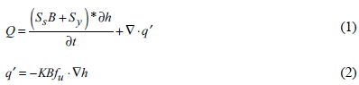
Here, q' is flow (m/s), Q is the volumetric flow (m3/s), Ss is the specific storage, B is the thickness in the saturated phreatic aquifer (m), Sy is the specific performance, K is the hydraulic conductivity tensor (m/s), f u is the function of viscosity and h is the hydraulic head.
A triangular two-dimensional mesh algorithm was used and mesh refinements in the river and well lines were carried out. Then, this mesh was projected in-depth to seven layers defined in the conceptual model, leading to six-nodes finite elements. The first layer was configured as a free aquifer. The code used for this mesh was developed by Jonathan Shewchuk at UC Berkeley, EE.UU (Shewchuk, 1997) and was used due to its high speed, and its ability to accommodate complex configurations of polygons, lines, and points.
The model was run in steady and transient states, adopting an Adams-Bashforth scheme for the latter. The Adams-Bashforth outline permits to control automatically the time-step scheme, providing an easier convergence and stability in model executions (Trefry & Muffels, 2007). In the transient model, the steady state model groundwater hydraulic loads were used as initial conditions. The system of symmetric equations (flow Simulation) in stable state was solved with the algebraic multigrid SAMG method (by K. Stüben, FhG-SCAI). This method is sharper for stable state models and simulations with a variety of element sizes. SAMG internally analyzes the best method and applies a CG (Conjugate gradient method) or SAMG (Algebraic multigrid) type solution. For the transient state, PCG (preconditioned conjugate gradient) method was used. Although the direct method assures a better model stability, the demand for memory and execution time for models with more than 100 thousand nodes, is not applicable.
The objective function ф is defined to iteratively optimize the model parameters (Carrera, Alcolea, Medina, Hidalgo, & Slooten, 2005; Medina, Galarza, Carrera, Jódar, & Alcolea, 2001). This optimization is expressed by measuring the objective function (Equation 3).
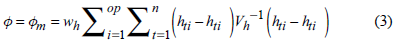
Here, i is the number of observation points (OP), PP or CZ, t is the observed time interval, h* is the hydraulic head vector at the observation points, h is the simulated hydraulic head vector, V h the covariance matrix, W h is the observations weights which has a value of one in our problem.
For ф m estimation, PEST was applied. Nonlinear PEST software (Model-Independ Parameter Estimation) developed by John Doherty (1994), uses an inverse code. PEST executes the simulation software iteratively by adjusting the parameters values to be estimated until the errors between the observed and simulated data reach the finishing criteria (Maheswaran et al., 2016; Woodward et al., 2016). The parameter search is carried out using the GLM algorithm (Gauss-Levenberg-Marquardt). This method linearizes the state variables dependence on the model parameters, while imposing a change on the parameter ∆p k for each iteration (Equation 4) (Finsterle & Kowalsky, 2011; Yao & Guo, 2014).
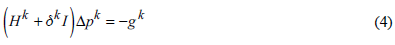
Here, H k represents an approximation of Hessian matrix of ф. g k is the gradient in the model parameter vector in * iteration /, is the identity matrix and δ k is the Marquardt parameter.
After each iteration, the model parameter vector is updated. Before consolidating this step, it is checked if the vector parameters components by iteration meet the assigned upper limit. This process is iterative until: 1.) if ф
i
. ≤0.0001, where ф is the OF value at the end of the optimization iteration ith, 2.) when 30 is the maximum number of optimization iterations, 3.) if
 ≤ o 1, where ф
min
. it is the lowest OF reached so far. For the development of this model, was established as convergence control numeral 1.
≤ o 1, where ф
min
. it is the lowest OF reached so far. For the development of this model, was established as convergence control numeral 1.
To evaluate the model performance, statistical measures were taken to quantify the differences in observed and simulated groundwater heads. In the present study, were used the coefficient of determination (R2), the mean square error (RMSE) and mean absolute error (MAE) (Carrera et al., 1993; Nash & Barsi, 1983; Sahoo & Jha, 2017; Muhammad Usman, Liedl, & Kavousi, 2015).
Study Area
The results are explored within a regional flow model that presents high hydraulic conductivity and is under the effects ofthe Inter-Tropical Convergence Zone, which characterize meteorological and hydrologic features. A domain of 17,000 km2 was defined in the central area of MMV, Colombia (Figure 1). The average amount of rainfall overpasses 2000 mm/year, and the main river has an annual average flow of2361 m3/s. The average annual temperature is higher than 24°C throughout the territory, and the terrain elevation varies between 16 and 3110 m.a.s.l (Ideam, 2014). The study area presents a high geological complexity, with variable depths in all the hydrogeological units. Its formation took place during the Tertiary, at the time of high volcanic activity of the Central Cordillera (Mojica & Franco, 1990). Result of this geological background, the area is tilted towards the East, having a monoclinal structure, disturbed by some folds and faults (Servicio Geológico Colombiano, 2014). It occupies a structural depression that is considered a half graben tilted towards the East, where it limits with inverse faults such as Salina (Ingrain, 2012). In general, rocks lean monoclinally from the Cordillera Central towards the Eastern Cordillera, but they are interrupted in-situ by faults and bends. At this basin, recent clastic sediments of alluvial type and sedimentary rocks of Quaternary and Tertiary age developed. The main characteristic of this material is the low consolidation and sediments predominance such as sand and gravel, interspersed with finegrained materials. In the MMV basin, groundwater is extracted from units that function as an aquifer. These units are recent alluvial and terrace deposits that emerge in the Magdalena River proximity with an average productive thickness of approximately 150 m (Gallego, Jaramillo, & Patiño, 2015) whose origin is associated with this body of water, and with the Mesa and Real Formations unconsolidated detrital sediments (sandstones, conglomerates).
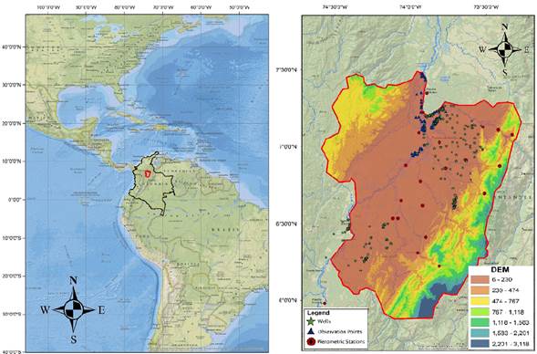
Figure 1 Location of influence area in the model (red). In addition to this the figure shows the locations of piezometric levels, Limnimetric stations, and Wells
The underlying rock represented at the East limit is used as a vertical and lateral no-slip boundary condition for every aquifer formation, which is not continuous through the whole domain. The following aspects were taken into account for the conceptual model integration: i) the relationship between each formation material, ii) homogeneity of hydraulic properties for regional scales, iii) an electrical resistivity analysis for each formation material, and iv) common permeability values. At a regional scale, the geological reinterpretation of the study area led to a simpler model of the hydrogeological basin. It included the depth of sedimentary formations, the Salina-Buitima fault, and every main fold. In addition, interpolation algorithms were used including secondary information from seismic and magnetotellurics studies, superficial geological interpretations, and stratigraphic from drilling well. In the end, seven layers resulted from this exercise, each one separated from the other by lithological contacts or erosive surfaces. Near-surface formations are considered the most important given the current water resource exploitation from those aquifers.
Data Sources
To describe a three-dimensional groundwater flow model geometry, it required a digital elevation model (DEM). It was obtained from SRTM satellite data derivation with a 30 m resolution between the coordinates 6° 7' 46'' N and 74° 39' 47'' W and an average vertical altitude error of 6.2 m (90% accuracy level) and a geolocation error of 9 meters for South America (Sharma, Tiwari, & Bhadoria, 2011). The recharge was obtained through a prior semi-distributed hydrological model consolidation: TopModel, whose information may be reviewed in (Arenas-Bautista et al., 2017). The piezometric levels and wells were obtained from the National Underground Water Forms (FUNIAS), compiled specifically for the national inventory of groundwater led by the Regional Autonomous Corporations (CAR). From that point on, geographical location information and type of points were collected. Water well pumping tests were obtained from the hydrogeological studies developed by Ideam and the National University of Colombia (Arismendy, Salazar, Vélez, & Caballero, 2004; Betancur et al., 2009), and the production blocks known as Guane (Ingeniería Geotec, 2016) and VMM-39 (Ecopetrol, 2016). The rivers levels for both steady and transient conditions were taken from the Ideam, limnimetric stations available in the area. Additionally, it became necessary to obtain the bathymetry and bed river level to consolidate the model input data. The geo-statistical model was defined by the transmissivity variogram in the model domain. The soil texture details for different depth profiles were available from well logs that were used to establish the initial values of different hydraulic parameters in each zone (Freeze & Cherry, 1979). The methodology used to generate the geological profiles and the consolidation of hydrogeological units is described in (Pescador-Arévalo, Arenas-Bautista, M. C., Donado, Guadagnini, & Riva, 2018).
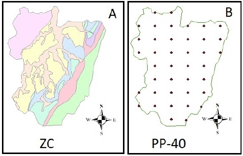
In the model development, eight constant zones were defined which correspond to the geological zones defined in the study area (Figure 2A). As opposed to the CZ technique, the PP method allows to estimate fields of continuous parameter distribution. The fundamental principle of this constraint is to prefer homogenous distributions of parameters whose values show as small a deviation as possible from those expected. In a geological context, a PP should preferably have a similar value to its neighbors within a certain distance. This distance and the strength of correlation are defined through a semi-variogram. In this research, due to the study area does not have sufficient and reliable data throughout the domain, and the available data are pooled in small areas of the study area, was decided to generate the PPs with uniform distribution. The model ran 50 times, and in each run the PPs were distributed so that their locations were different (x, y, z), but the space between them was constant. It means that a rectangular pattern was used for every run, but the PP locations changed after every run, always keeping the same pattern (Figure 2B). The random location of PPs with a uniform distribution allowed to represent without bias the locations that had no field measurements in the calibration process and the post-calibration analysis identified the parameter contributions to the uncertainty. The variogram that defined the spatial behavior of PP's was an exponential model, with a range of 2000 m and a variance of 2 without nugget effect. The K values obtained vary from 10-5 to 35 m/day. We defined 167 observation points based on the piezometric levels (Figure 1), because all piezometric data levels registered in FUNIAS were taken on different dates, and it was not possible to find records of continuous time series monitoring for these measurements. An average data level was used as reference in the numerical model in steady state. For transient state, a measurement grouping by month was made. This grouping assumes that levels in the same months of different years, exhibit a similar behavior due to the results of the hydrological processes analysis. Finally, a series of monthly data was consolidated for an average year. The extraction data comes from 78 independent pumping tests in the wells where information was found within the model domain (Figure 1). Pumping rates range between 10-2 m3/day and 250 m3/day.
Conceptual Model
Figure 3A represents the conceptual application model area. The zone is limited to the east and west by the limits of SAVMM aquifer system that acts as an impermeable barrier due to its igneous-metamorphic nature (Ideam, 2014). The South and North limits of model act as an inflow and outflow, respectively, in the different zone sections. The groundwater flow is estimated by Darcy's law (Karay & Hajnal, 2015; Şen, 2015) using piezometric data, and is generated in south-east to north-west direction. The elevation in the focus zone descends smoothly in south-north direction, conserving the properties of an alluvial valley and, therefore, provoking a regional movement of underground water throughout this depression (Ingrain, 2012). Additionally, there is a register of low scale domestic and industrial use of groundwater collection obtained with pumping equipment (Gonzalez, Saldarriaga, & Jaramillo, 2010). Most recharge of groundwater occurs at the mountain ranges, from rainfall infiltration, and at the low-lands, from channel drainage losses. The region weather is mainly semiarid with high temperatures, especially during dry season, which causes a loss of water in the form of evapotranspiration (Asociacion Colombiana del Petroleo, 2008).
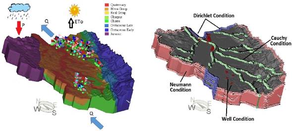
Figure 3 Hydrogeological Conceptual Model. 3A-Represent the conceptual model of influence area. 2B-Show the boundary conditions used in the model.
The hydraulic properties of the aquifer system make possible to identify areas with primary and secondary porosity and characterize them as units able to store and transmit water with relative ease. The horizontal (x axis) permeability is an order of magnitude higher than the vertical (Han & Cao, 2018; Xie, Hu, Jiang, & Liu, 2006). The system total porosity ranges between 25% and 3%, with an average specific yield of around 14%. The test holes pumping results and the lithological analysis allow us to conclude that the hydraulic conductivity varies from 20 m/day to 0.1 m/day
Numerical Model
The recharge was estimated with a one-year time scale, taking proportions from average monthly data ranging from 12 years, between 2000 and 2012. The information was consolidated on a spatial scale of 6 km x 6 km resulting from hydrological modeling (Arenas-Bautista et al., 2017). The recharge is assigned as a material associated property, which becomes variable in time for transient model (Figure 4). The loading boundary conditions (Figure 3B) were assigned as a first type variable Dirichlet condition in south and north edges from the model domain, according to water level historical records. For the seven consolidated rivers in the model domain a Cauchy boundary condition was applied. This requires the hydraulic conductance of the riverbed material and its geometry procurement, which were obtained establishing the initial conductivity from the pumping tests and the cross-section geometry, supplied by the limnmetric stations in the area. The East and West model limits were conditioned by the application of Neumann boundary conditions; given they are considered as a watershed. The inlet and outlet flow sections and the model domain flow were identified using piezometric water level contours, and applying Darcy's law. Finally, pumping wells were assigned as a well edge condition where a defined extraction was applied to a node.
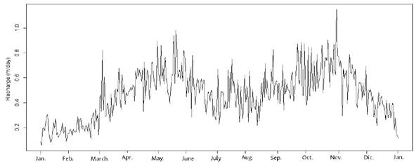
Figure 4 Recharge data used in the transient model. This series was built for an average year, based on result of the hydrological model (Arenas-Bautista et al., 2017).
For CZ application a pattern on materials disposition according to the hydrogeological units was defined. For the PP, it was observed that it was not possible to obtain a defined pattern for the same materials, so the information was spatialized. For this, the PP spatial distribution model of the hydraulic properties used Kriging (Tsai & Yeh, 2011). This technique was used given its additional use for regularization processes, which are based on the same variograms used for regionalization (Janetti, Riva, Straface, & Guadagnini, 2010; Kashyap & Vakkalagadda, 2009; M. Riva, Guadagnini, Neuman, Janetti, & Malama, 2009; Tsai & Yeh, 2011). For the development of this model, each layer was treated as a single zone and tested with a variable number of PP to evaluate the response model. The principle of parsimony establishes that the numbers of parameters considered in an estimation process must be kept to a minimum (Golmohammadi, Khaninezhad, & Jafarpour, 2015; Merritt, Croke, & Jakeman, 2005; Tonkin, Doherty, & Moore, 2007). However, when PP are used in conjunction with regularization, this number tends to increase (Panzeri et al., 2012).
In order to check the results from the calibration process, an uncertainty analysis was performed. In this analysis, some basic metrics are reported such as RMSE, Pearson correlation and NASH efficiency coefficients.
Results and Discussion
The two calibration processes (CZ and PP) are compared briefly in their value parameters, model fit and predictions. This comparison focuses on the model ability to simulate the real system and to show conceptual differences. The model residuals respect to the observation points allows us to infer that model calibration allows to adequately represent the assumptions presented in the conceptual model, both in the CZ and in the PP technique (figure 5A). The average residual differences in PP results is lower than 1 m. the CZ technic exhibits oddment points between 1 and 3 m. The possible reason for these mayor differences would be associated with the large number of wells in this region, which pumps extensively the groundwater. Therefore, the possibility of an occasional partial inflow across the study area boundaries, especially on the eastern and western boundaries, could not be well represented by the input/output flow limits conditions. The error obtained in the observation points is summarized in table 1. These results include R2, MAE and RMSE. The value of R2 for the calibration model is 0.99; likewise, MAE, which is an efficiency of calibration indicator, is 0.25. Figure 5B allows to evidence optimal simulation results, as the observation values are adequately represented under the numerical model assumptions, and the figure 6 presents the results of transient-state calibration. The hydrographs of simulated versus observed heads over time show a relatively good match between observed and simulated heads, even if the model tends to overestimate the piezometric levels. The general behavior of PP technique offers average values of 142 m in the OF. However, the results obtained in CZ show a variation of 6 m above the results with respect to values obtained from PP. These results are in agreement with the findings of (Andrés Alcolea et al., 2006) where it is concluded that the PP technique offers better results for the analysis of heterogeneity.
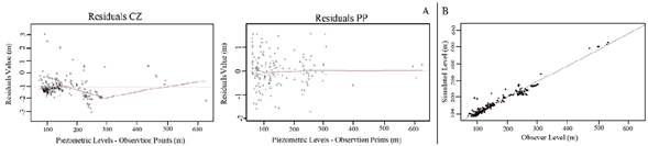
Figure 5 Result of the conceptual model from the residual values of the numerical model. 5A-shows the model residual respect to the observation points in the CZ and PP techniques 5B-shows the result of graphical fitting of observed and simulated heads at the observation points.
Table 1 Experiment description and result of the statistical metrics
| Experiment | Description | фm | фr | ф | MAE | RMSE | R2 |
|---|---|---|---|---|---|---|---|
| CZ | 8 geological units: Quaternary, Mesa, Real group, Chuspas, Chorro, Cretaceous early and late, Jurassic | 145.36 | 178.58 | 323.94 | 0.25 | 0.93 | 1 |
| 40 | 40 PP | 114.27 | 159.37 | 273.64 | 0.25 | 0.81 | 1 |
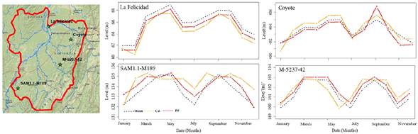
Figura 6 Results of observed and simulated levels in the model for trasient state. The results are shown for dour wells (the most representatives in the area): Felicidad, Coyote, SAM 1.1 and M-5237
The hydraulic conductivity analysis (Figure 7) in the model shows that, in the Quaternary, the average Kx values in CZ is different from the average PP values. This occurs because of the lack of knowledge of hydraulic properties of outcrop geological units in the zone. The most information and monitoring compiled for this model has an 80 m depth (for Mesa and Real formations); because of this, the model representation fits with higher certainty. In the seven (7) remaining model units, the Kx values assignment does not represent a direct link either with CZ nor different PP. This may be due to the ignorance of depths of hydraulic properties higher than 600 m. Additionally, the scarce available information is focused on specific influence areas, which gives another struggle for its representation. Finally, results show that in the deepest model units equifinality issues can arise when the same model performance with a different parameter for the same node is generated.
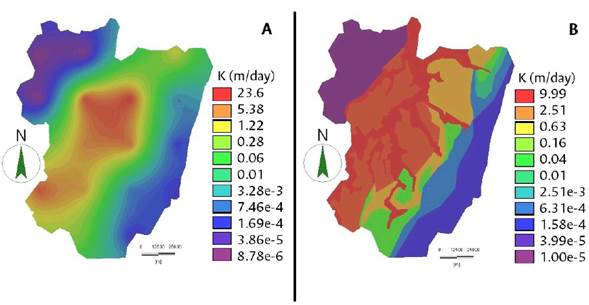
Figure 7 Result of K in the proposed hydrogeological model 7A. The model developed with PP. 7B. The model developed with CZ.
Additionally, is evident a strong separation of the Quaternary aquifer and Mesa formation with values of 10 m/day and 2.5 m/day respectively. It is evident in Figure 7, that the PP calibration process presents a K three times higher than the CZ model. In general, the K values for all hydrogeological units are within the reported range in literature. Comparing the two methods evaluated through the CZ and PP, they show similar model characteristics: i.) The East and West regions of the model, corresponding to Jurassic and early Cretaceous units, have a uniformly low conductivity, which corroborates the conceptual model assumption establishing those zones as water divide, ii.) The model presents small areas of high conductivity in the north and central part and, iii.) The highest conductivity is found in Quaternary and Mesa formation. An interesting fact is that the estimated field begins to reflect some large known scale geological structures also perceived on the CZ model. The storage does not significantly influence the hydraulic head during the one-day simulation period. Therefore, it can be concluded that K is the only definitive parameter in hydraulic head modeling and that each parameter is sensitive, and does not depend on other parameters.
In summary, compared to the previous CZ technique, PP approach is not only able to provide satisfactory matches for all measured heads and reproduce large-scale and local features of the measured groundwater level, but it can also extract more information of heterogeneity at several scales using the same amount of measured information. All the results shown above indicate that the PP approach provides a more realistic model to simulate river-groundwater interactions based on parameters. Taking into account the parameters calibrated in both techniques, the ratio between the horizontal and vertical hydraulic conductivity is at the center of its range with a value of around 0.1. Therefore, the vertical flow in the aquifer is ten times slower than the horizontal flow that coincides with the regional dips (sub-horizontal layers)
Conclusions
This article has been focused to identify if there are biased parameters in the model solution and determine the heterogeneity of the hydraulic properties by applying a calibration scheme based on CZ and PP techniques in tropical basins. Subsequently, the optimized model has been used to quantify the groundwater flow through topographic boundaries.
The analysis of the PPs used for estimation of hydraulic parameters offers a guide to estimate the heterogeneity in hydraulic anisotropic conductivity in unconfined aquifers. The regional groundwater model provided information within regional flow patterns. The flows through all internal limits constitute 3 to 16% of their discharge and are significant in relation to pumping; therefore, it is important to consider these flows in hydrological models, since they could have a great impact on the water currents simulation. Additionally, this highlights the need for flow models (surface and underground) coupled on a regional scale due to most surface water models assume zero flow between topographic divisions. The use of real data as initial aquifer parameters reduces the interactions necessary to minimize ф, improving potential estimates and estimating the possible convergence.
The inverse model results in the calibration process demonstrated a better response in the real representation of the system. The hydraulic head error was reduced by 3% compared to the conceptual model developed. Although the minimum square error of the state variable was minimized at the observation points, the model validation showed consistent results at the control points. This idea supports the model solution, showing that the model calibration through the PPs is more robust and flexible in contrast to the CZ parameterization given its lower subjectivity and lower of the heterogeneity representation of the hydraulic properties. In conclusion, the research results indicate a less significant pattern for the CZ method compared to the PP-based model. Therefore, to identify the spatial value of the observations there must be a certain degree of flexibility and variability in the parameterization of the model.
Although the PP method reduces the homogeneity produced by CZ, it has some limitations, e.i., to overlook other sources of model error and result in an over-parameterization or equifinality. An important uncertainty of the PP method is the choice of the number and location of the PPs, as well as the effect it has on reducing the variability of the parameters in the model during the investment problem. Although there is no defined guideline for generating these points, the results of this article indicate that better results can be obtained using a uniform pattern, reducing the spaces between them which is useful to correlate the hydraulic properties as a guide for the separation distance. In the same way, the interpolated fields of K resulting from the application of the PP method work properly for the estimation of the flow at the regional scale; however, it can lead to significant limitations for other applications, such as solute transport modeling.
Finally, these results are the basis for the identification of biased parameters and the heterogeneity of hydraulic properties when a variable amount of the PP number is used. Additionally, based on the results obtained, is proposed to evaluate the model plausibility to determine if this can improve the identification of the heterogeneity of K and if it would be sensitive to the amount of PPs.

