


 English (pdf)
 Article in xml format
 Article references
 Send this article by e-mail
 Cited by SciELO
  Cited by Google
  Similars in
SciELO
Similars in
SciELO  Similars in Google
 Permalink
Introduction
In China's oil census and exploration, gravity and magnetic exploration have played an important role as a pioneering means of exploration. However, due to the rapid development of seismic exploration technology since the 1970s, gravity and magnetic technology were once at low tide (Metcalfe et al., 2015). As a new force in comprehensive geophysical exploration of petroleum, since the 1980s and 1990s, oil and gravity have revived the glory, and it has made due contributions to oil exploration in the new era. At present, China National Petroleum Corporation and Sinopec Group have established many exploration new areas in the west and central regions (Beck et al., 2015). The common features of these new areas are as follows: First, the surface conditions are very complex, including mountains, deserts, wind erosion landforms, and loess cover; second, the geological and geophysical conditions are complex. Multi-phase tectonic movements, multi-stage magmatic activities often cause the complexity of underground geological structures. Pleated and reversed napped structures abound, and the physical properties of rocks vary. These complex and unique surface and underground conditions in China have brought severe challenges to seismic exploration, and seismic data collection is difficult. Excited reception conditions are poor, the signal-to-noise ratio is low, and even effective seismic signals are not obtained, which greatly affects the exploration pace of the new area.
The gravity and magnetic exploration technology have always been characterized by lightness, speed, low investment, and high efficiency. In the early exploration of the new area, it can play an important role in delineating the distribution of faults and igneous rocks, the division of tectonic units, the study of the basement structure, and the discovery of local structures. It can provide the basis for deploying seismic exploration (Babak et al., 2015) and can complement or partially replace where seismic exploration is difficult. In the past decade, many exploration areas in the western, central, and southern regions have been or are working on gravity and magnetic exploration and have achieved results. Zhang Xuejian et al. extracted the seismic wavelet from the depth domain offset profile and then used the convolution formula to obtain the depth domain synthetic record. Considering the difference between the upper and lower speeds of the interface, Ma Jinfeng follows the time-domain convolution formula and replaces the time domain seismic wavelet with the wavelet operator in the depth domain. That is, the depth domain asymmetric wavelet operator is used to obtaining the synthetic record. In this paper, gravity and magnetic exploration techniques are used to obtain information on complex topography in the Tongbai basin such as the basement structure, the distribution of sedimentary rock series, and the distribution of fault systems (Jokela & Ramallo, 2015). On this basis, the fine horizon calibration technology can maximize the use of all data in complex areas to ensure that the formation and reservoir calibration is relatively accurate in the whole and full sections. Finally, the fine calibration of the petroleum underground layer in the Tongbai basin is realized.
Materials and methods
Research area overview
Tongbai basin is a small inter-mountain fault basin in the eastern Qinling fold belt. The terrain is hilly and semi-mountainous, rivers, gullies, etc. The previous small scale weight and magnetic survey results show that the regional heavy magnetic field is seriously disturbed, which makes the wild construction and abnormal geological interpretation has certain difficulties. The main body of the Bouguer gravity anomaly in the survey area is a complete gravity low zone with the shape of "Yuanbao" sitting south to the north, with a relative gravity value of at least -10.5mGal, and its center is located near the Yuehe store; the anomalous line of the anomalous center is circular, and the two wings are lifted outwards to the northwest and the north. The west, north, and east of the survey area are three high-gravity belts, and the high gravity belt in the north is wedged from the northwest to the southeast, whose relative gravity value is +29mGal. Gravity step belts with different strikes and scales and isomorphic twisted belts with equal anomalies are covered with survey areas, such as the Shilipu-Xuzhai gravity step belt in the northwest direction and the same-line twisted belt in the eight-acre land as Shenpu. Under the background of the strong gravity gradient, the local gravity anomaly shows weak, and it can be distinguished abnormal bulge gravity of Lizhuang, Niejiaxiahe, and Shenpuyizhongwan. These characteristics of Bouguer gravity anomalies reflect the uniformity of the survey area in the regional structure, but the complexity of the fault structure and local structure. The upward extension of the gravity anomaly is similar to the basic characteristics of the Bouguer gravity anomaly. The residual gravity anomaly reflects the internal structure of the basin very finely. One of its characteristics is to divide the gravity low zone centered on the Yuehe store into two completely trapped gravity belts in the south and north. In Shenpu-Wang Laozhuang domain it has a beam, dividing the southern main gravity low zone into two negative anomalies in the east and west, and the negative anomaly zone in the west is in the orchard area, whose size and amplitude are much smaller than those of Yuehe store in the east. The northern subtropical low-band center is located between Shangmazhuang, Baishuyuan, and Louzi Shangzhuang. It is separated from the southern part of the main gravity low belt by the Niejiaxia River. Another feature of it is that it clearly reflects seven gravitational step bands, such as the eight-acre land in the northwest and the Wuzhuang gravity step belt.
Establishment of gravity and magnetic geological model
The gravity-magnetic fine-measurement (I) profile coincides with the Wuhedian-Wucheng earthquake survey profile. The seismic profile has poor reflection quality, and the geological horizon of the seismic interface needs to be further determined. To this end, the gravity geological model needs to be constructed. The construction of the initial gravity geological model is mainly based on the results of seismic interpretation (Foster et al., 2015), and refers to the ground geological and drilling data. The density of each layer is given according to the actual measurement and statistical results. The modification and forward modeling of the model uses the second-degree gravity anomaly human-machine dialogue interpretation program, and the interpretation results are shown in Figure 1.
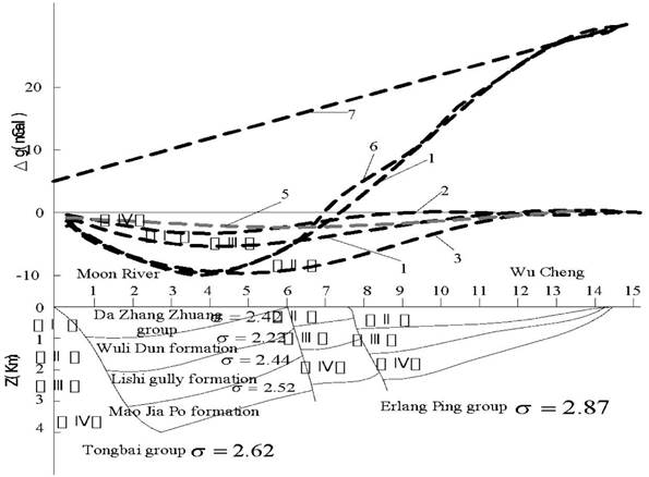
The number 1 represents the measured Bouguer gravity anomaly; 2 represents the calculated value of the Dazhangzhuang group (I); 3 represents the calculated value of the Wulidun group (II); 4 represents the calculated value of the Li Shigou group (III); 5 represents the calculated value of the Maojiapo group (IV); 6 represents the calculation of the total gravity anomaly value; 7 represents the regional gravity field value.
The following three points are recognized through forwarding modeling:
(1) The model is modified several times without considering the influence of the regional field. The calculated value in the south of the profile is always a few milligrams larger than the Bouguer anomaly. According to the regional field characteristics reflected by the Bouguer gravity anomaly map of 1:500,000, after the region anomaly with the gradient of 1.478mGal/km is removed, the satisfactory fitting result is obtained (Primack, 2015). It can be seen that the existence and change of the regional gravity field in the basin cannot be ignored.
(2) The Wulidun group is the largest in terms of reflecting the negative anomalies in the basin, followed by the Lishigou group, the Dazhangzhuang group, and the Maojiapo group. The Wulidun group is 2-6 times that of the Maojiapo group. Obviously, the variation of the thickness of the Wulidun group is the main geological factor causing gravity anomalies.
(3) In the forward calculation, the base density of the basin is taken uniformly, which is 2.67g/cm3. As a result, regional positive residuals appear in the northern half of the profile, while regional negative residuals appear in the south. The northern basement is taken as the Erlangping group (density 2.67g/cm3), and the southern basement is taken as the Tongbai group (density 2.67g/cm3). The fitting effect is ideal. It can be seen that there is a change in the lithology of the basement in the basin (Qayyum et al., 2015).
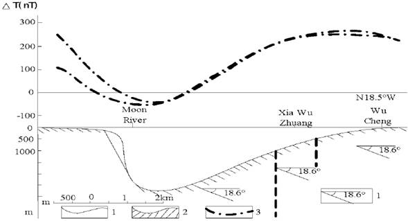
The magnetic initial geological model refers to the interpretation results of the seismic survey profile. The value of the base magnetism is derived from the actual measured and statistical data, and the abnormal inversion results are referenced. Model modification and forward calculation use a combined model human-machine dialogue interpreter. The final interpretation results are shown in Figure 2. In the forward modeling process, the uniform magnetic substrate is used. As a result, the theoretical anomalies and measured anomalies in the south of Xiawuzhuang Village are well fitted, while the theoretical anomalies in the northern part are much lower than the measured anomalies. Thereafter, the base magnetic value of the north of Xiawuzhuang is relatively good, and the theoretical anomaly can be well fitted with the measured anomaly. It can be seen that the lithology of the basement of the basin does change. The southern part may be the mixed granite or the rock with the same magnetic properties, while the northern part is a more magnetic type.
Inversion of bedrock depth
There are three difficulties in the inversion of the bedrock depth in this basin:
(1) The gravity exploration work for the purpose of studying the basement structure of the basin is the first time in this area. Due to the limitations of objective conditions, the density data is not sufficient, especially the lack of density data of the lower three strata with depth changes;
(2) The Maojiapo group overlying the basement has large buried depth and a small difference in density from the base (Mavrommati et al., 2017);
(3) The scope of work is small. At present, most of the existing interface inversion methods are based on the forward modeling, and there is inevitably an area loss. In view of this situation, the exposed areas of the bedrock at the edge of the work area are known as known points. Taking the entire lower three systems as the equivalent density layer, according to the measurement, the density of the equivalent density layer is calculated to be a = 2.43g/cm. The ParkerR.L. method without loss of area is used in the calculation to obtain the gravity anomaly inversion result.
There are many methods for calculating the buried depth of a magnetic body by using magnetic anomalies. The method of calculating the buried depth of a magnetic body by computer requires that the magnetic anomaly is isolated, obvious and the interference is small, or the depth of the base is up and down at an average depth. If the characteristics of the magnetic field and the base undulation of this area cannot meet the requirements of the above algorithm, it is difficult to obtain a good effect. To this end, we use the tangent method that has been tested by practice and adopt corresponding algorithms for the anomalies of different characteristics. A total of 187 depth points are calculated, and they are distributed uniformly in the measurement area, which can satisfy the drawing of the magnetic bedrock depth map.
According to the results of gravity anomaly inversion, the range of bedrock exposure is basically consistent with the distribution range of geological outcrops; the depth of bedrock in U13 well is 900m, and the inversion result of bedrock depth is 920m. The depth of the U27 well is 963m, which is close to the bottom boundary of the Wulidun group. The inversion results show that the bedrock depth is about 1500m. The northwestern, eastern, and southern parts of the survey area are all within 100m, and the actual situation is basically matched. The U13 well is located on the gentle slope of the magnetic base, between the isobaths of 900m-1000m; the U27 well is located on the steep zone of the magnetic base, between the depth lines of 1200m-1300m. The above results indicate that the inversion results of the gravity and magnetic anomalies can better reflect the depth and undulation of the basin basement (Yan et al., 2016), which has been confirmed by the later completed area seismic exploration data.
Analysis of factors affecting horizon calibration
Fine-level calibration on the basis of high-precision gravity and magnetic survey and the influencing factors to be considered are important topics in the calibration of horizons. In order to achieve fine horizon calibration, it is necessary to combine geology and earthquake, and comprehensively use geological data, logging data, seismic data, and VSP data. The specifics should include the accurate application of the seismic reference plane and the core elevation, the application of the logging curve, and the selection of the frequency.
Accurate application of seismic datum and core elevation
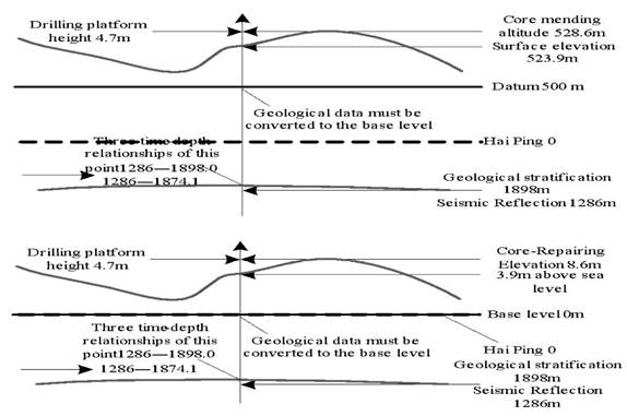
Figure 3 shows the effect of the core elevation on the calibration. It can be concluded from Figure 3 that the core elevation is indispensable data information, and the information must be correct, and the ground elevation cannot be used instead of the core elevation. The relationship between these aspects is correct and the time-depth relationship established in the calibration is correct. Otherwise, the accuracy of the time-depth relationship is low or the relationship between time and depth is wrong (Zhang et al., 2017).
Application of logging curve
(1) Check the added curve with the curve observer, check the original data for the problematic curve, and then add it again after finding the cause.
(2) Look at the AC curve (porosity curve) whether the sand and mudstone velocity can be separated (Lei et al., 2014). Generally, due to compaction, the sandstone velocity may be lower than that of mudstone. In addition, the sandstone has a reduced velocity after oil and gas.
(3) If there is no AC curve (porosity curve) or AC curve (porosity curve) is not good, the time difference curve can be converted from the induction curve.
(4) Multi-curve analysis and comprehensive analysis of the strata, which has a better understanding of the well, making the calibration better.
There are eight methods for correcting the logging curve, and they are divided into three categories: manual mode correction, log curve processing, and VSP correction.
(1) Manual correction
The manual correction method is divided into the following four editing methods:
a. Table format editing. The method mainly performs point-by-point editing correction on the peaks (ie, singular values) in the logging curve.
b. Square wave editing. In the specified depth interval, this method provides four methods for modifying the amplitude of the logging curve by the new average method, the multiplier method, the offset method, and the constant value method.
(I) New average method. A constant offset is added to all amplitudes within the selected depth range of the log curve so that the new average amplitude value matches the given average.
(II) Multiplier method. Multiply the amplitude value for a given depth range by a constant multiplier (Zhou, 2018).
(III) Offset method. A constant value is added to the amplitude of each point in the selected depth range in the acoustic time difference curve.
(IV) Constant value method. The amplitude value of each point in the selected depth range in the acoustic wave time difference curve is set to a constant value.
(V) Thickness editing. Editing functions such as stretching, compressing, and deleting a segment of the log are provided.
(VI) Mouse editing. Mousing over the existing curve is drawing a new curve value.
(2) Filter processing
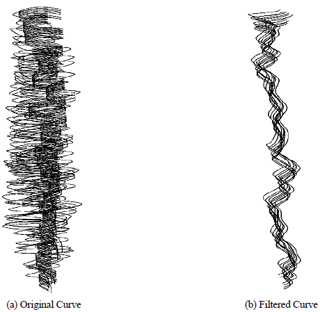
In the logging curve filtering process, we mainly use the median filtering and bandpass filtering methods to eliminate the singular points in the curve and achieve the purpose of smoothing the curve. The actual application effect is taken as the U13 well: after we filter the logging curve, the logging curve becomes smoother and has no singularity. Figure 4 (a) is the original logging curve, and Figure 4 (b) is the filtered logging curve. It can be seen that after filtering, some singular points in the curve have been filtered out to achieve a smooth curve.
(3) VSP correction
The VSP correction includes two methods: global correction and time difference correction:
(1) Overall correction. The error is obtained by using the VSP seismic data and the overall acoustic logging data to obtain an error curve, and then the error curve is used to correct the original acoustic wave logging curve.
(2) Time-division difference correction. This method only performs time difference correction on a certain section of the logging curve.
Set a critical value ∆t min, when the sound wave propagation time value is below ∆t min, it is considered reasonable, no correction is needed; when the sound wave propagation time value is greater than the critical value ∆t min , the part exceeding the propagation time is multiplied by the factor G, the formula can be expressed as:

In formula (1), ∆t cor is the original sound wave propagation time value; ∆t min is the artificially set threshold (threshold value); G is the ratio of the drift point value to the sum of the sample difference values contributing to the drift.
The synthetic seismic record calculated using the U13 well logging curve without VSP correction is shown in Figure 5(a), and the synthetic seismic record calculated by the VSP corrected logging curve is shown in Figure 5(b). Comparing, it can be seen that the in-phase axis that is not obvious before the correction is more obvious after the correction process, and it is in good agreement with the actual seismic profile.
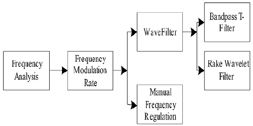
Frequency selection
It can be seen from Figure 6 that based on the frequency analysis, the filter is used to adjust the frequency, or the frequency is manually adjusted, and the band-passing T-filter and the Lectra wavelet filter can be selected when the filter is adjusted to obtain the synthesized recording frequency. The recording frequency must match the seismic frequency.
Underground layer calibration method
The above process determines the depth and undulation of the basin base by high precision gravity and magnetic exploration technology. Therefore, the petroleum subterranean geological structure or rock layer properties are studied, so as to carry out calibration of the petroleum underground layer through the horizons division, time-depth transformation, and geological layer determination of the rock formation.
Layer division
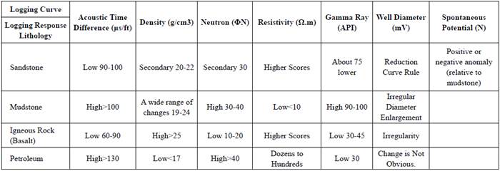
Dividing a rock formation with multiple well logs is much more reliable than dividing the horizon by acoustic time difference alone. Moreover, in the case of no core section, the lithology of the reflective layer can be accurately determined. The available logging curves include seven parameters: acoustic time difference, density, neutron, resistivity, natural gamma, natural potential, and well diameter. The influence of each logging curve on lithology is shown in Table 1.
In the layered calibration, the thin layer selection and lithology grading are handled by the following two principles:
(1) The division of the thin layer should consider the difference in speed between the thin layer and the adjacent layer and the thickness of the thin layer itself. High-speed thin layers and low-speed thin layers with large speed differences should be retained, while thin layers with small speed differences can be considered to be rounded off smoothly (Song, 2017). For the thickness of the thin layer, after the time-depth conversion, the low-speed thin layer on the depth axis can be converted into the thickness on the time axis. The highspeed thin layer on the depth axis is converted into the thin layer with very small thickness after being converted into time. Considering the above situation and the workload of artificial stratification, the minimum thickness of the layer is given: 1) the depth difference is greater than or equal to 4m when the highspeed thin layer is high; 2) the depth difference is greater than or equal to 2m when the low-speed thin layer is used.
Time-depth conversion
In order to facilitate the time-depth conversion, equal-depth interval interpolation is performed on the layered average time difference and density, and the interpolation interval is 1m. The two-way travel time sequence corresponding to the horizon depth sequence can be expressed by the formula:
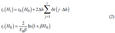
Where V 0 = 1830m /s;β = 0.00034m-1; H 0 represents the starting depth of the processing of the well data. Using equation (3), we can find the velocity sequence and density sequence with the two-way travel as variables for each depth difference. They can be expressed as:
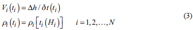
The above velocity and density sequences are not equally time-interval. For this reason, the above sequence is linearly interpolated by 2ms to obtain velocity sequences and density sequences of equal time intervals.
Geological horizon determination
In the case of unified drilling geological horizon and reliable seismic velocity, the geological horizon method for determining seismic reflection is relatively simple. The geological horizon of the seismic reflection layer can be determined by simply comparing the seismic reflection layer with the geological horizon by synthetic recording. However, in the case where the geological stratification of the survey area is not uniform, the method of strict seismic reflection layer tracking, high-precision speed analysis (Jiang & Ma, 2017), and various synthetic records for geological horizon reliability test can accurately obtain the determination and unification of the seismic geological horizon.
(1) Geological horizon of the seismic section
The synthetic record is compared with the geological horizon. First, the polarity of the seismic data needs to be determined, followed by the type of seismic wavelet. According to the regulations of the International Geophysical Society, the collection of seismic data in the field is always negative, that is, the single gun records the first arrival wave and jumps down. Most of the domestic oil fields are consistent with this, but some oil fields are the opposite. It is stipulated that the single-shot records the first arrival of the wave, that is, the acquisition polarity is positive. The wavelet shape of the airborne airgun is fixed and is the minimum phase; the wavelet excited by the ground explosive source is also the minimum phase. According to this, the seismic data collected in the field is the positive phase profile of the minimum phase, and the data collected in the offshore field is the negative phase profile of the minimum phase.
The valleys of the reflected in-phase axis on the negative polarity section correspond to the regular reflection coefficient, and the peak corresponds to the negative reflection coefficient. The peak of the reflected in-phase axis on the positive polarity section corresponds to the regular reflection coefficient, and the two-valley corresponds to the negative reflection coefficient. When the composite record is compared with the horizon, for the reflective layers with the positive reflection coefficient, the synthetic record with the same polarity is consistent with the horizon of the seismic profile. For reflective layers with a negative reflection coefficient, the synthetic records with different polarities are also consistent with the seismic profile horizon.
According to the above principle of horizon comparison, the paper compares the synthetic record with the horizon of the U13 well on the 75.6 line and the U27 well on the 90.5 line. The comparison results of the two wells are shown in Table 2.
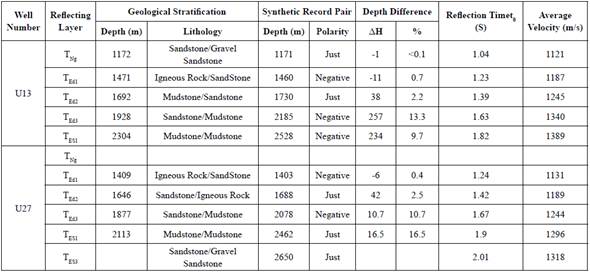
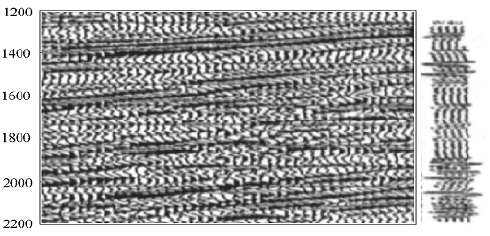
From the comparison of the horizons, it can be seen that the polarity of the seismic reflection is consistent with the combination of the lithology above and below the geological interface. That is, the positive polarity of the reflection corresponds to the geological interface that is thin on the top and thick on the bottom. The geological interface corresponding to the negative polarity of the reflection is the opposite. The calibration of the synthetic record of the U13 well on the line profile is shown in Figure 7. The reflection horizon on the profile corresponds well to the ankle in the synthetic record.
(2) Inspection of layer reliability
In the case of inaccurate or inconsistent geological horizons, the back- calculation speed of the horizon data is mainly used, and the reliability of the horizon is judged according to the regularity of the velocity distribution (Lian et al., 2017). If the average velocity of the seismic reflection layer is accurate, the horizon determined by time-depth conversion of the reflection layer is reliable; on the contrary, if the synthetic recording depth is correct, the speed variation law based on the back-calculation of the layer data must be reasonable (Yang et al., 2020).
According to the reflection time t0and depth h of the U13 well and U27 well after the horizon comparison, the average velocity V of each horizon is inversely calculated from shallow to deep. Then, the curve of the average velocity as the function of depth is made, and the velocity curves of the wells are plotted in the same coordinates, as shown in Figure 8.
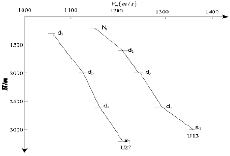
As can be seen from Figure 8, the curves are developed in the lateral direction and are nearly parallel to each other. The horizon of the U13 well formation is at a high position and the speed is high. The U27 well is located at a low position with low speed. This change in velocity coincides with stratigraphic fluctuations indicating that the horizon determined by synthetic records is reliable (Wu et al., 2020).
Results
In the experiment, the Nanyang oil field in the Tongbai basin appeared as an example. The U13 well on the 75.6 line, the U27 well on the 90.5 line, and the inclined well B2 on the 82.3 line were selected as experimental objects to verify the practicality of the method in calibrating the petroleum underground layer (Cheng et al., 2020).
Distribution and combination characteristics of the faults system
The Tongbai basin is controlled by the northwest and northeastward boundary faults, and the northern part of the basin is uplifted in the late period and is denuded to form the braided basin with characteristics of south deep and north shallow. According to the gravity and magnetic anomaly characteristics and the bedrock depth map, 14 basement faults were inferred, which can be divided into 4 groups according to the distribution characteristics. Gravity and magnetic exploration were carried out on the Tongbai basin by this method. The geological results of gravity and magnetic exploration are shown in Figure 9 (Gao et al., 2018).
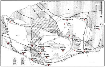
(1) Faults in the northwest direction. There are 7 faults in this group, which are the main faults in the basin, and most of them are the extension of the northwestward deep faults in the Qinling fold belt in the basin. They are Bamudi-Niejiaxiahe faults (F1), Tongbai (North)-Chuanshan store faults (F2), Tongbai (South)-Shilibao faults (F3), Wucheng-Huangzhuang faults belt (There are 4 northwestward faults F4, F5 F6, F7,) in the belt. Among them, F2 and F3, constitute the stepped edge faults of the southwestern margin of the basin (Gao et al., 2019).
(2) The faults in the northeast direction, the Chushandian-Caodian (F14), and F2 and F3 played the controlling role in the formation of the basin.
(3) Faults near north-south direction. This set of faults controls the substructure of the basin depression and the tectonic pattern of the eastern stepped uplift belt. They are Shenzhuang faults (F ), Caodian-Bashuyuan faults (F), Huangqi-Guxian town faults (F13), Maojiapo faults (F8), Wanglaozhuang-Xuzhai faults (F9), and Dajizhuang - Jinqiao faults (F10 ). Among them, these three nearly parallel staircase faults play an important role in the evolution of the basin (F11, F12, F13). F8 forms the boundary between the bulges and depressions in the western part of the basin. F9 and F control the bulge of the Golden Bridge.
(4) Near East-West faults. There may be a fault in Wucheng-Guxian Town, which is the extension of F7 to the east. It constitutes the boundary between the basin depression zone and the northern uplift zone.
It can be seen from the distribution and combination characteristics of the above faults that the northwest and northeast faults jointly control the formation of the basin, while the near north-south faults play the controlling role in the later evolution of the basin.
Horizon calibration of electrical and lithological information
The B2 in Nanyang Oilfield is an inclined well. To make full use of the electrical and lithological information of the well, the method is used for horizon calibration. Firstly, the orientation and well deviation of the different well sections of the B2 are segmented and interpolated. The spatial coordinate values are obtained by the above equation and the time-depth relationship of the well, and the position of the target layer on the seismic section is found. Figure 10 is the positional view of the target horizon of the B2 on the plane, and Figure 11 is the positional view of the target horizon of the B2 on the section. Through the calibration of the method, the corresponding relationship of the target horizon on different seismic sections is established to achieve the purpose of stereo calibration. The method in this paper can intuitively perform the calibration work in the vertical direction. The three curves of the acoustic time difference, density, and natural potential of B2 are digitized, and the dip angle and well deviation data are input to the workstation, and segmentation interpolation is performed. The log is corrected to the vertical direction by the above equation. In the production of synthetic records, using the logging speed of the well or adjacent well, the converted acoustic curve is subjected to depth correction to complete the calibration of the logging curve. Figure 12 is the comparison of the synthetic records of the B2 and the seismic traces produced by the method of the present invention. It can be seen from Figure 12 that the synthetic records made using the corrected log curves have good correlation with the seismic traces.
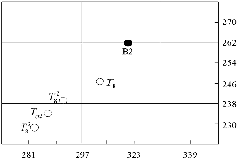
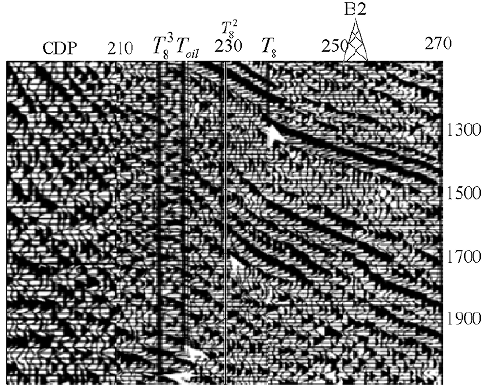
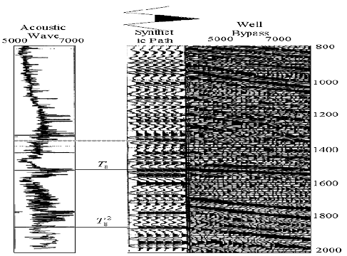
Figure 12 The synthetic record of well B2 and the contrast map of parallel seismic trace produced by this method
The method can be used for the horizon calibration of inclined wells. The method is not only suitable for anisotropic media, but also suitable for strata with a less lateral variation of lithology in local strata. It is more flexible and can be corrected by using various velocity data.
Calibration method
Figure 13 and Figure 14 show the depth domain synthetic records of the seismic profiles between the U13 and U27 in Nanyang Oilfield. Figure 13 is the synthetic seismic record made with asymmetric wavelets and Figure 14 is the synthetic seismic record made with wavelets extracted by autocorrelation analysis. Qualitative comparison of synthetic seismic records and crosswell seismic profiles can be obtained from two methods. It can be seen that they are in good agreement and can be used for horizon calibration between wells.
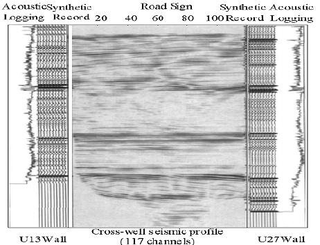
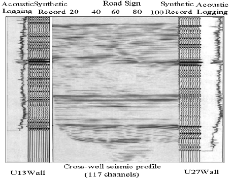
Figure 14 Synthetic records of wells U13 and U27 produced by wavelets extracted by autocorrelation analysis
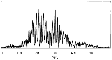
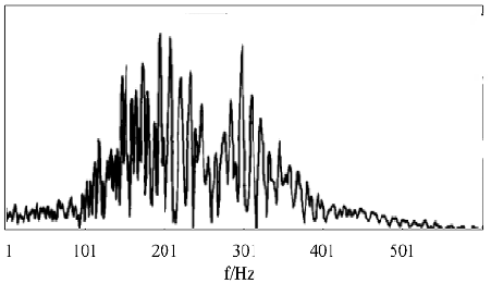
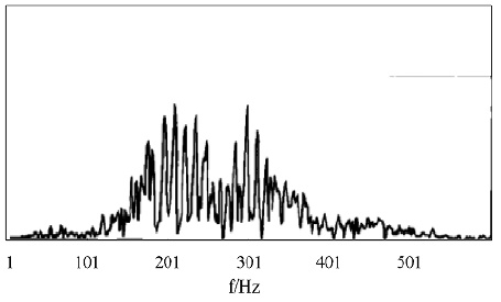
The near well is compared with the synthetic records produced by the two methods in terms of a spectrum. Figure 15 shows the spectrum recorded by the U27 well. The effective frequency range is 30--550Hz, and there is a relatively low-value area of the spectrum around 280Hz. Figure 16 is the spectrum of the synthetic record of the U27 well fabricated by autocorrelation wavelets, the morphology of which is similar to that of Figure 15. Only the amplitude of the low-frequency region is relatively large, and the main frequency moves slightly in the low-frequency direction. Figure 17 shows the spectrum of the synthetic record of the U27 well made with asymmetric wavelets, which is quite different from the difference of Figure 15. Such as shape near 280Hz, in the low-frequency region, and in high-frequency region, but its main frequency is relatively high, and the frequency band is relatively narrow. Therefore, in the actual calibration of petroleum underground layers, the active records produced by the autocorrelation method can be used to achieve horizon calibration.
Discussion
(1) High precision gravity and magnetic exploration: Petroleum geophysical exploration in small basins is often constrained by many factors. However, improving the economic benefits of oil and gas exploration and speeding up exploration are two important factors. The Tongbai Basin is representative of the Lower Tertiary Basin in the eastern part of China. It is now used as an example to discuss the petroleum geophysical work procedures in the small basin. The high precision gravity and magnetic exploration of the Tongbai basin basically identified the basement structure of the basin, the distribution of sedimentary rock series, and the distribution of the faults system, and its effect in finding local structures is particularly prominent. The local structures reflected by the local anomalies of gravity and magnetic fields are confirmed by subsequent seismic exploration data. In addition, small basins generally have poor topographical conditions, and deep and shallow geological conditions are often more complex than large basins. The gravity and magnetic exploration are much more serious than the difficulties encountered in seismic exploration. In view of the above situation, we believe that in the oil and gas exploration of the Lower Tertiary small basin, the reasonable procedures for petroleum geophysical exploration should be divided into the following steps:
The first step is to carry out high precision gravity and magnetic exploration with less investment, quick effect, and good effect. The working scale is not less than 1:50,000 and the density of measuring points is not less than 8-10/Km3. The total accuracy of several gravity anomalies is not less than 10uGal, and the magnetic measurement accuracy is not less than ±2.0nT. The second step is to arrange regional two-dimensional seismic lines according to the interpretation results of gravity and magnetic anomalies, so as to improve the regional exploration of the basin and verify the interpretation results of gravity and magnetic anomalies. The third step: using the acquired seismic data, the gravity, and seismic data are comprehensively processed to further develop the geological information of high-precision gravity and magnetic data. The interpretation results of gravity and magnetic anomalies are extended to the entire basin, and favorable areas containing hydrocarbons and favorable local structures are identified. The fourth step is to arrange two-dimensional or three-dimensional seismic exploration on favorable local structures, carry out structural detailed investigation, implement traps, and provide drilling well locations.
(2) Marking of the petroleum underground horizon: As can be seen from the above, there is a certain error in the time between the reflective layer on the time section and the corresponding reflective layer in the synthetic records. In the inverse calculation of the average velocity curve, it is also possible to observe the deviation of individual points from the average line. The main reason for the difference between the two is that the reflection on the synthetic records is the normal reflection, and the reflection on the time profile is in-normal reflected; the reflective layer on the synthetic records and the reflective layer on the time profile are not in the same section when the formation is tilted. The position of the reflective layer on the time profile is laterally offset and laterally offset. The depth of the reflective layer is the apparent depth, which does not correspond to the vertical depth of the reflective layer on the synthetic records section. The sonic velocity used in synthetic records is different from the actual seismic velocity in the time profile, where the sonic logging data is corrected without influencing factors. The reflective layer on synthetic records is the subwave with constant frequency and amplitude and is superposed by the sequence of reflection coefficients. In the reflective layer on the time profile, the frequency and amplitude of the wavelets vary with depth. It can be seen that the reflection layer on the synthetic records and the reflection layer on the time profile can correspond exactly only after the factors causing the above errors are eliminated. In general, it is inevitable that there is a certain error in the horizontal comparison of synthetic records. In addition to technical reasons, in areas where sand-shale interbeds are developed, seismic reflection is the superposition of thin-layer reflections, and there is no clear geological horizon corresponding to the seismic horizon. Sometimes, since a reflected wave group is controlled by multiple formations, it is also possible that the subsequent phase of the reflected wave group corresponds to a certain geological interface.
Conclusions
The calibration method of the petroleum underground layer based on high precision gravity and magnetic exploration is researched in this paper.
Firstly, the high-precision gravity and magnetic exploration technique are used to explore the Tongbai basin. It basically finds out the basement structure of the basin, the distribution of sedimentary rock series, and the distribution of faults systems, and its effect in finding local structures is particularly prominent. Based on the survey of the basement structure of the basin, the distribution of sedimentary rock series, and the distribution of the faults system measured by high precision gravity and magnetic exploration, the calibration of petroleum underground horizons is realized by stratigraphic division, time-depth conversion, and horizon determination. The calibration method of petroleum underground horizons based on high precision gravity and magnetic exploration can not only accurately survey complex underground rock formations, but also accurately calibrate the petroleum underground horizons. This lays the theoretical foundation for the future oil mining industry.

