Maximum Likelihood Classification of Soil Remote Sensing Image based on Deep Learning

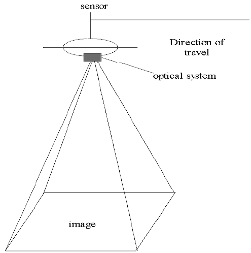
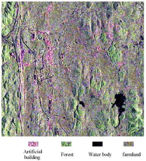
Soil remote sensing image is a kind of soil remote sensing image obtained by various sensing devices (such as radar, camera, scanner, etc.). Its acquisition principle process is shown in Figure 1, and the form of the obtained remote sensing image is shown in Figure 2.

Figure 1 Principle of soil remote sensing image acquisition 

Figure 2 Remote sensing images 

The obtained soil remote sensing images can accurately identify and classify soil types, make soil maps, and analyze soil distribution law, which brings great convenience to soil survey. To improve the classification quality of soil remote sensing images, this paper studies a more effective classification method, which combines deep learning with maximum likelihood estimation to make up for each other's shortcomings (^{Fitak & Johnsen, 2017}).

The research on maximum likelihood classification of soil remote sensing images based on deep learning is mainly divided into four stages: the first stage is to preprocess the soil remote sensing images acquired by remote sensing equipment; the second stage is to detect the targets of remote sensing images by using deep learning algorithm and extract the classification features of various soil images; the third stage is to classify the soil remote sensing images based on the methods mentioned above by using maximum likelihood estimation method. In the fourth stage, the performance of maximum likelihood classification of soil remote sensing images based on deep learning is tested by an example to ensure the effectiveness and practicability of the method (^{Handelman & Chor, 2017}).

Preprocessing of Soil Remote Sensing Images

As shown in Figure 2, the quality of the original soil remote sensing image is not high, which is not conducive to the subsequent image classification. Therefore, it is necessary to pre-process the image before classification to improve the image quality, including image graying, image denoising and image correction (^{He et al., 2018}).

(1) Image graying

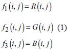
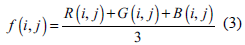
Grayscale image, commonly speaking, is the conversion of a color image to a gray image whose pixel value is between 0 and 255. The whole image is composed of different degrees of gray. Its purpose is to reduce the interference of color to the target information in the image. There are four main methods of gray image processing: component method, maximum method, average method, and weighted average method, as shown in Table 1.

Table 1 Four methods of image graying 

Method	Definition	Formula	Explanation of parameters
Component method	Taking the brightness of three components in a color image as the gray value of three gray images, a gray image can be selected according to the application needs.		f k (i, j)(k = 1, 2,3)is the gray value of the converted gray image at (i, j); R, G, and B represent color components, ranging from 0 to 255
Maximum method	The maximum brightness of three components in a color image is taken as the gray value of a gray image.	f (i,j) = max[R(i,j),G(i,j),B(i,j)] (2)
average method	The three-component brightness of the color image is averaged to get a gray value.
weighted average method.	According to the importance and other indicators, the three components are weighted averaged with different weights.	f (i,j)= 0.30R(i,j) + 0.59G(i,j) + 0.1L9(i,j) (4)

(2) Image denoising

Influenced by natural factors such as illumination, cloud, and equipment itself, the original remote sensing image collected contains a lot of noise. After graying, it can see that there are many white elements on the image. These elements are image noise, as shown in Figure 3.

Figure 3 Image noise 

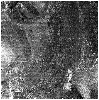
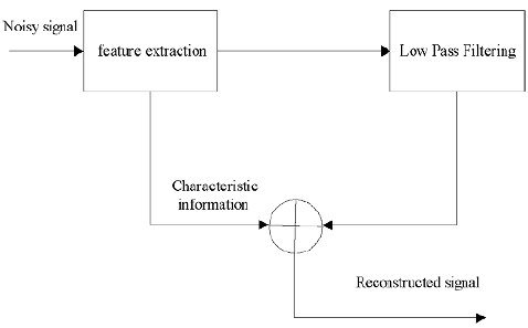
The existence of image noise will blur the image target and reduce the image quality, so it needs to be de-noised. At present, denoising methods include mean filtering, median filtering, wavelet transform and neighborhood averaging. Wavelet transform is a commonly used method at present (^{Li et al., 2017}). The basic principles are as follows: the multi-scale wavelet transform is performed on the noisy signal, and the wavelet coefficients belonging to the noise are removed at each scale, and the wavelet coefficients belonging to the signal are preserved and enhanced. Finally, the wavelet transform is used to restore the original signal, so that denoising is achieved, as shown in Figure 4.

Figure 4 Wavelet denoising 

(3) Image correction

In the acquisition process of soil remote sensing image, besides the image quality degraded by noise, it will also be affected by the characteristics of the sensor itself, the illumination conditions of the ground objects (topography and solar altitude angle) and the atmospheric effect, which will lead to the inconsistency between the measured values of remote sensing equipment and the actual spectral emissivity of the ground objects, i.e., radiation distortion. The radiation distortion will then cause the geometric position, shape, size, orientation and other features of the original image to deviate from the expression requirements in the reference system, that is, geometric distortion (^{Ma et al., 2018}). In view of the above two distortion phenomena, it is necessary to correct and restore the image.

1) Radiation distortion correction. According to the three causes of radiation distortion, i.e. the characteristics of the sensor itself, the illumination conditions of the ground objects and the atmospheric effect. The calibration of the remote sensor, the solar altitude and the terrain, and the atmospheric correction are carried out by these three methods, respectively, as shown in Figure 6. Sensor calibration: in order to eliminate the radiation error caused by the sensor itself, the dimensionless DN value recorded by the sensor is converted into the atmospheric top radiation brightness or reflectance with practical physical significance.

Topographic correction: it can mainly reduce the shadows in remote sensing images, because it restores spectral information, but because the existence of shadows will make the image stereoscopic, which is a visual experience. To see whether topographic correction improves image quality, it depends on whether spectral information has been corrected. Cosine correction and semi-empirical C correction are usually used for topographic correction (^{McCord et al., 2017}).

Atmospheric correction is divided into statistical model and physical model according to the correction principle. The statistical model is based on the correlation between surface variables and remote sensing data, without knowing the atmospheric and geometric conditions of image acquisition. It has the advantages of simplicity and less parameters.

2) Geometric distortion correction. Geometric correction refers to the elimination or correction of geometric errors in remote sensing images, which mainly involves three processes: selection of control points, transformation of spatial position (coordinate transformation) and resampling of pixel luminance resampling (^{Pritikin et al., 2018}).

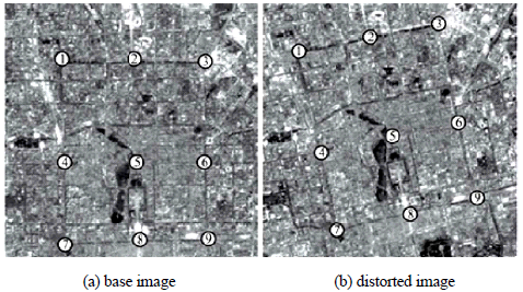
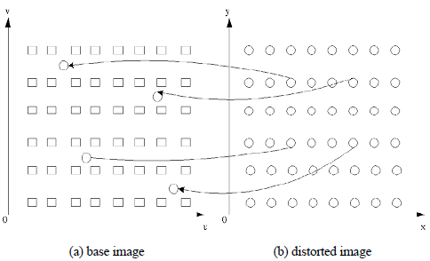
Control point selection: Firstly, two remote sensing images are selected, one is the reference image and the other is the geometric distortion image, as shown in Figure 5. A certain number of control point pairs on the above two images are selected. The selection principles are as follows: the selected control points should be obvious in the remote sensing image of soil; the objects covered by the control points are always fixed; the selected control points have the same topographic height on the two images; the control points should be evenly distributed in the image; and the number of control points should not be less than 5.

Figure 5 Control point selection 

Space position transformation (coordinate transformation): the purpose is to find the correct coordinates of the object. There are two main methods at present, direct method and indirect method. Direct method, as its name implies, calculates the coordinates of each pixel in the image to be corrected in turn by the coordinates of the control points on the reference image, as shown in Figure 6.

Figure 6 Direct method 

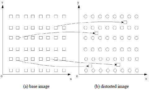
The advantage of the direct method is that the coordinate values of each pixel calculated in the image to be corrected will not change. The disadvantage of the direct method is that the distribution of pixels will not be uniform.

In contrast to the direct method, the indirect method calculates the coordinates of each pixel on the reference image from the image to be corrected. The schematic diagram is shown in Figure 7.

Figure 7 Indirect method 

The advantage of the indirect method is that it can ensure the uniform distribution of the corrected image pixels in space (^{Temmer et al., 2017}). The disadvantage of the indirect method is that the row number of the relocated pixels is not an integer relationship with the original image, so the pixel value of the original image needs to be re-sampled.

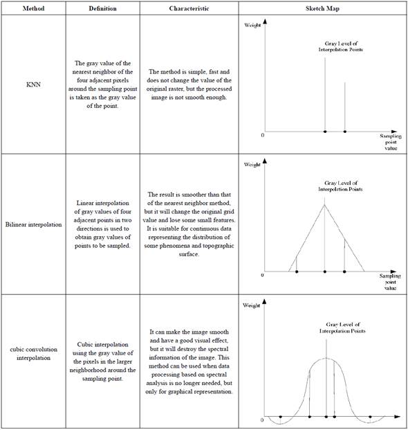
Pixel luminance resampling: resampling refers to assigning the pixel value of the original image to the corrected image according to a certain relationship. At present, there are three main methods for resampling pixel luminance values: nearest neighbor method, bilinear interpolation method and cubic convolution method, as shown in Table 2.

Table 2 Resampling method of pixel luminance 

Target Detection of Soil Remote Sensing Image based on Deep Learning

On the basis of the above, this chapter uses a deep learning algorithm to detect the target of soil remote sensing image, extract soil characteristics, and prepare for subsequent classification. Deep learning belongs to a branch of machine learning. It is an algorithm based on an artificial neural network to represent data. Therefore, before analyzing deep learning, it is necessary to understand artificial neural networks (^{Wang et al., 2017}). Artificial neural network (ANN) is an abstract arithmetic model developed to simulate the process of processing information by human brain neurons. It consists of a large number of nodes (or neurons) connected with each other, as shown in Figure 8.

Figure 8 Artificial neural network 

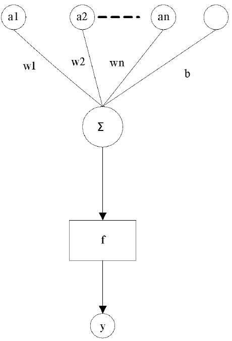
In Figure 8, a is a signal other than the neuron; w1 to wn is the weight of the signal transmitted to the neuron; b is the bias of the signal; f is the excitation function, generally a non-linear excitation function such as sgn symbolic function or sigmoid type continuous function, and y is the output of the neuron.

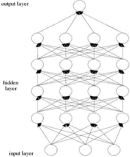
Artificial neural networks consist of an input layer, hidden layer and output layer. When input layer neurons are stimulated by input signal, the activation function of neurons in the hidden layer is stimulated. When a certain threshold is reached, neurons are activated and output signal is generated through the output layer (^{Xu et al., 2017}). On the basis of this structure, it is proposed that deep learning is a deeper artificial neural network, which consists of multiple neurons stacked together, as shown in Figure 9.

Figure 9 Deep artificial neural network 

There is a special network structure in deep learning, namely convolution neural networks. It is a kind of feedforward neural network with deep structure including convolution calculation (^{Zhao et al., 2018}). Its structure consists of input layer, convolution layer, pool layer, full connection layer and output layer. The structure is shown in Figure 10.

Figure 10 Convolutional neural network 

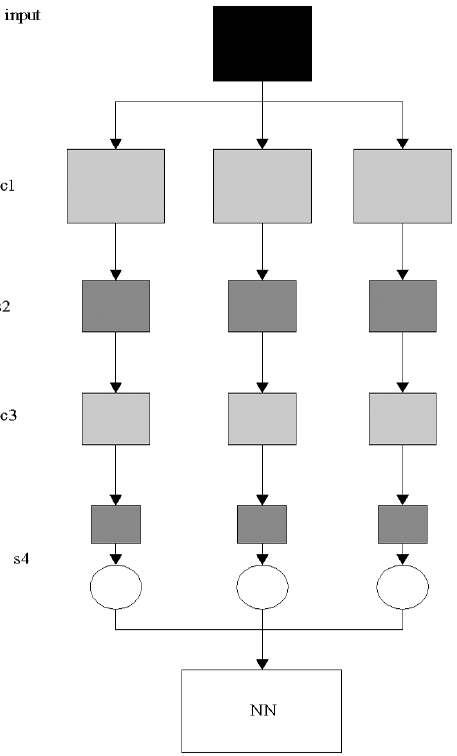
The basic principle of convolution neural networks is that the input image is convoluted by three trainable filters and additive bias. After convolution, three feature mapping maps are generated at layer C1. Then four pixels of each group in the feature mapping map are summated, weighted and biased, and three feature mapping maps at layer S2 are obtained through a Sigmoid function.

These maps are filtered to get layer C3. This hierarchy produces layer S4 again, as does layer S2. Finally, these pixel values are rasterized and connected into a vector input to the traditional neural network to get the output (^{Zhu et al., 2019}).

Based on the above convolution neural network, the object detection and extraction of soil remote sensing images are carried out. The specific process is as follows:

(1) Convolutional neural network training

Step 1: Select the remote sensing image of soil for training as the input sample of the model.

Step 2: Set the weights between layers, the thresholds of output units and hidden units to random values close to 0, and initialize the accuracy control parameters and learning rate of the model.

Step 3: Take an input mode X from the training group and add it to the network, and give its target output vector D.

Step 4: Calculate an intermediate output vector H and the actual output vector Y of the network.

Step 5: Compare the element y_K in the output vector with the element dk in the target vector, and calculate M output error terms.

Step 6: Calculate L error terms for hidden elements in the middle layer.

Step 7: Calculate the adjustment formula of each weight value and the adjustment formula of threshold value in turn.

Step 8: Adjust weights and thresholds.

Step 9: When k goes through 1 to M, judge whether the index meets the accuracy requirement: E<e, where E is the total error function. If not satisfied, go back to step 3 and continue iterating; if satisfied, go to the next step.

Step 10: At the end of the training, save the weights and thresholds in the file. At this time, it can be considered that the weights have been stabilized and classifiers have been formed. When training again, the weights and thresholds are directly derived from the file for training without initialization.

(2) Realization of soil remote sensing image detection

Step 1: Use the trained convolution neural network to extract image texture features, and convolution calculation is carried out to obtain image feature map.

Step 2: Make sampling of the feature map of soil remote sensing image by using adaptive pooling model

Step 3: Merge the feature map into a column of feature vectors, and input to the full connection layer. Update the weights of the network filter through label data back propagation algorithm.

Step 4: Finally, the feature column vectors are input into softmax to complete the object extraction of soil image.

Classification of Soil Remote Sensing Image based on Maximum Likelihood Estimation

Maximum Likelihood Classification (MLC) has a rigorous theoretical basis. It is easy to establish a class discriminant function with normal distribution. It combines the mean, variance and covariance of each category in each band. It has good statistical characteristics and has been considered as a more advanced classification method.

In traditional remote sensing image classification, maximum likelihood method is widely used. This method obtains the mean and variance of each category by statistics and calculation of the interested region, and then determines a classification function. Then each pixel in the image to be classified is substituted into the classification function of each category, and the category with the largest return value of the function is regarded as the category of the scanned pixels, so as to achieve the classification effect. Its basic principle process is as follows:

Step 1: Determine the area to be classified and the number of bands and feature classifications to be used, and check whether each band or feature component has been positioned with each other.

Step 2: According to the ground condition of the typical area, choose the training area on the image.

Step 3: Calculation of the parameters. Calculate and determine the prior probability according to the image data of the selected training areas.

Step 4: Classification. Substitute the image pixels outside the training area into the formula one by one. For each pixel, it is calculated several times in several categories. Finally, the size is compared, and the largest category is selected.

Step 5: Generate a classification map and specify a value for each category. If each category is divided into 10 categories, it is determined that each category is 1, 2, 10. The classified pixel values are replaced by category values. The final classified image is thematic image. Because the maximum gray value is equal to the number of categories, it needs to add different colors to all kinds, when displaying on the monitor.

Step 6: If there are many errors in the classification, it needs to re-select the training area and do the above steps until the results are satisfactory.

Based on the principle of maximum likelihood method, the process of soil remote sensing image classification is as follows:

Step 1: Preprocess the image;

Step 2: Initialize the number of classifications and training parameters to determine the number of data blocks and threads;

Step 3: Establish and initialize grid threads and the amount of data to be computed by each thread.

Step 4: Detect the connectivity of the network and grid nodes, and add a grid computing thread model to the grid;

Step 5: Each thread carries out cyclic grid calculation according to the sample's subset data, and all data in the grid unit are computed to get the category and stored to this node.

Step 6: Transfer the results from each grid site to the host computer, and merge the grid results.

Step 7: Release grid resources and output classification results to files.

Example Analysis

General Situation of Test Area

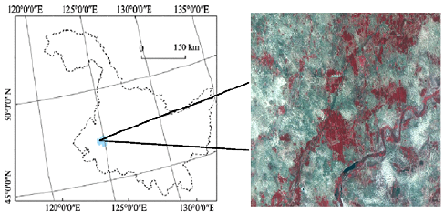
Lindian County is located in the western part of Heilongjiang Province, the hinterland of Songnen Plain, with an area of about 3 500 km². It belongs to Daqing City, Heilongjiang Province. It has a continental monsoon climate in the middle temperate zone. It is rainy and warm in summer, dry and cold in winter. Its geological structure belongs to the paleo-Asian tectonic domain. It has abundant wetland resources and natural rivers such as Uyur River and Shuangyang River. The elevation is low and terrain is flat, but micro-topography is more complex and low-lying leads to difficult drainage, which is easy to form marshes. According to the data of the second national soil census, most of the parent materials of the soils in Lindian County are loesslike deposits (^{Palagan & Geetha, 2016}). There are four main soil types (By the second national soil census). They are chernozem, meadow soil, marsh soil and aeolian sandy soil. Among them, chernozem accounts for more than 60% of the total soil. Chernozem is also an important part of black soil resources, and its organic matter content is high. Soil fertility is large, which is a very suitable soil type for grain production. The Landsat 8 OLI image of Lindian area on May 3, 2014 is selected for this test. The study area in the image is almost covered by clouds. In May, it is bare soil period. There is neither a large area of vegetation nor snow. It meets the research requirements of this paper for bare soil period, as shown in Figure 11.

Figure 11 Test zone 

Sample Training

Samples are divided into four categories: chernozem, meadow soil, marsh soil and aeolian sandy soil. There are 10 samples in each category and 80 samples in total. 40 samples are used for experimental training and the remaining 40 samples are used for testing. The parameters of the trained convolutional neural network are shown in Table 3.

Test Verification

In the trained model, the remaining sample data sets are input for a performance test, and the experimental results are expressed in the form of confusion matrix. Confusion matrix, also known as error matrix, is a standard format for accuracy evaluation, which is expressed in the matrix form of n rows and n columns. Specific evaluation indicators include overall accuracy, mapping accuracy, user accuracy and so on. These accuracy indicators reflect the accuracy of image classification from different aspects (^{Sato, 2012}; ^{Zhu, 2016}). Each column of confusion matrix represents the prediction category, and the total number of each column represents the number of data predicted for that category; each row represents the true belonging category of data, and the total number of data in each row represents the number of data instances in that category. The sum of each row represents the true number of samples for the category, and the sum of each column represents the number of samples predicted for the category.

There are 40 test sample data in this experiment, which are predicted to be four types (chernozem, meadow soil, marsh soil and aeolian sandy soil), each of which has 20 samples. After the three methods are classified, the confusion matrix is shown in Tables 4, 5 and 6.

Table 4 Confusion matrix of the classification results of the proposed method 

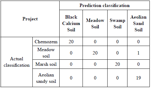
Table 5 Confusion matrix of classification results of soil remote sensing image classification method based on deep learning 

Table 6 Confusion matrix of classification results of soil remote sensing image classification method based on maximum likelihood estimation 

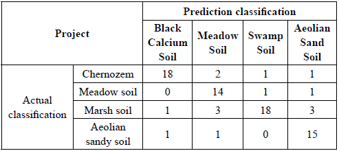
Comparing Tables 4, 5 and 6, it can be seen that after the proposed method is used to classify, 20 samples in the first, second and third rows of the confusion matrix established according to the results correspond to the first, second and third categories respectively, indicating that the samples are all correctly predicted, and only one sample belonging to the fourth category in the fourth row is misclassified into the second category. This result is much better than the other two methods, which shows that the performance of the proposed method is better.