English (pdf)
 Article in xml format
 Article references
 Send this article by e-mail
 Cited by SciELO
  Cited by Google
  Similars in
SciELO
Similars in
SciELO  Similars in Google
 Permalink
Nomenclature
α : Standard Penetration Test Blow Count Correction Coefficient with respect to Fine Content
β : Standard Penetration Test Blow Count Correction Coefficient with respect to Fine Content
∆ : Focal Depth
εv: Volumetric Strain
γ : Unit Volume Weight
σ, σ0: Total vertical stress
σ, σ0: Vertical effective stress
amax: Peak Ground Acceleration
Cn: Depth Correction Factor
Cb: Borehole Correction Factor
Ce: Hammer Energy Ratio
Cr: Rod Length Correction Factor
Cs: Correction Factor for Samples with/without liners
Cv: Factor to correct measured shear wave velocity
CPT: Conic Penetration Test
CRR: Cyclic Resistance Ratio
CRR75: Cyclic Resistance Ratio
CSR: Cyclic Stress Ratio
DR: Relative Density
FC: Fine Content
fs: Sleeve Friction
GUI: Graphical User Interface
h : Projection of the Earthquake Source to Earth's Surface
hw: Water Table Level
Ic: Soil Behaviour Type Index
M : Earthquake Magnitude
MJ: Earthquake Magnitude defined by Japan Meteorological Association
ML: Local Magnitude
MW: Moment Magnitude
MSF: Magnitude Scaling Factor
Nmea: Measured Standard Penetration Test Blow Count
(N1)60: Corrected Standard Penetration Test Blow Count
(N1)60FC: Standard Penetration Test Blow Count Corrected with respect to Fine Content
qc: Tip Resistance
qc1: Corrected Tip Resistance
qc1F: Tip Resistance Corrected with respect to Fine Content
Pa: Reference Stress of 100 kPa or about Atmospheric Pressure
rd.: Stress Reduction Coefficient
Rf: Sleeve Friction Ratio
SF: Safety Factor
SPT: Standard Penetration Test
Vs: Measured Shear Wave Velocity
Vs1: Corrected Shear Wave Velocity
z : Depth
1. Introduction
The assessment of the soil resistance against liquefaction or the amount of settlement of an engineered building caused by liquefaction is a remarkable phase concerning geotechnical and geophysical investigations. In earthquake-prone areas, during dynamic loading, i.e., an earthquake, pore water pressure increases in undrained and cohesionless soils. Therefore, these materials lose their solid behavior and act as if liquefied materials (Terzaghi and Peck, 1948; Ishihara and Yoshimine, 1992; Bekin and Ozcep, 2017). In general, the earthquake hazard risk increases because of liquefied behavior. Because of having great importance on engineered buildings and hence having a significant impact on natural hazards, researchers have studied the liquefaction phenomenon after the 1964 Niigata Earthquake.
From the fundamental theoretical background point of view, scientists have been proposed empirical relationships to determine the probable effects and to reduce the hazard levels based on liquefaction for more than 30 years. For example, Liao and Whitman (1986) have introduced the stress reduction coefficient (rd) to calculate the cyclic stress ratio (CSR). Youd and Idriss (1997) have presented a better way to compute CSR in their study. Andrus and Stokoe (2000) have formulated the relationship between the shear wave velocity (VS) and the cyclic resistance ratio (CRR). Youd et al. (2001) have demonstrated the relationship between CRR and corrected Standard Penetration Test (SPT) blow count numbers (N1)60. Tokimatsu and Seed (1987) have presented formulas to calculate the amount of expected settlement for liquefaction vulnerable regions dependent on (N1)60. Likely, Ishihara and Yoshimine (1992) have proposed empirical formulas for settlements with respect to (N1)60 values and corrected tip resistance (qC1) values of CPT.
The target of this study is to present a deterministic liquefaction analysis routine, soiLique, with a graphical user interface (GUI). This routine is the first MATLAB® based soil liquefaction analysis routine. The program presented in this study, soiLique, includes several approaches for the assessment of the maximum extent of liquefaction-susceptible areas. Firstly, Kuribayashi and Tatsuoka (1975), Wakamatsu (1991), and Wakamatsu (1993) that have related Mj., and the maximum distance for the liquefiable area (R). Although Liu and Xie (1984) have used ML, Ambraseys (1988) have made use of Mw for the estimation. Additionally, Ulusay et al. (2000) have proposed the relation between MS and the maximum distance R.
The results of soiLique were compared to the liquefaction analysis panel of another program, SoilEngineering, introduced by Ozcep (2010), to test the robustness of the algorithm. It is a widely used -especially in Turkey-, free access, and user-friendly Microsoft Excel® based program for the geotechnical and geophysical analysis of soils. It provides the user to prepare data, to derive parameters, and to carry out analysis of geotechnical and geophysical problems. The fundamental characteristic of soiLique is its independence from MATLAB®. In other words, soiLique can be used without MATLAB® by installing MATLAB® Runtime Environment v9.7 to run.
In the present study, the theory associated with soiLique is explained in the second chapter. The third chapter focuses mainly on the framework of soiLique. In the fourth chapter, the geological setting of the study area, where the real data are collected, and the analyses for checking the robustness of soiLique are presented. In addition to the tables and plots presented in the results and discussion section, readers can find some plots and more detailed tables in the supplementary file.
2. Theoretical Background
The theory associated with soiLique is explained in this section. There are various approaches and assessment methods to conduct a solution-oriented liquefaction analysis. Analyses that are mentioned in the present study can be classified as the assessment methods for the maximum extent of a liquefiable area, the calculations of settlements or prospective settlements, and liquefaction safety factor. These theoretical principles are represented in three sub-sections. In the first one, approaches of the maximum distance of a liquefiable area are explained. After that, safety factor analysis, including CRR75 (Cyclic Resistance Ratio, subjected to Mw=7.5) and CSR (Cyclic Stress Ratio), calculations are presented as the second sub-section. In the next sub-section, calculations of the settlements triggered by liquefaction are explained. Lastly, a simple analysis method, which has been introduced by Tezcan and Teri (1996), is explained.
2.1. The Evaluation of a Maximum Extent of a Liquefiable Area
Several investigators have studied the spread of liquefaction during former earthquakes and proposed the relationship between the magnitude of an earthquake, M, and the maximum distance from the epicenter to the liquefied area, R. Liquefaction prone areas can be estimated immediately from the magnitude of the predicted earthquake with the help of these approaches if the seismic activity in the corresponding area is known from the historic earthquake catalog.
Kuribayashi and Tatsuoka (1975) have shown the relationship between magnitude and maximum epicentral distance to a liquefied site by using 32 historic Japanese earthquakes. The logarithmic relation can be expressed as:

where MJ is the earthquake magnitude scale defined by Japan Meteorological Association, R denotes the distance, in km, between the earthquake epicenter and the farthest liquefied site in km. Liu and Xie (1984) have proposed another relationship based on the Chinese liquefaction database concerning the local magnitude (ML) :

where ML is the earthquake magnitude defined by Richter (1935), and R is the maximum distance, in km, of the liquefied site to the epicenter.
Ambraseys (1988) has represented two different approaches to estimate the seismic moment magnitude (Mw) from a distance between the epicenter and liquefied site. In the first approach, Ambraseys (1988) has standardized the Equation 3 for shallow and intermediate-depth earthquakes. According to the study, earthquakes having intermediate-depths and the much longer duration of shaking may induce liquefaction at distances greater than those dictated by shallow-focused earthquakes. The data points Re and Mw are bounded by the equation:
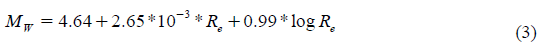
where Re is the maximum epicentral distance, and Mw is the seismic moment magnitude. In the second approach, Rf is the closest distance from a shallow seismic source of the furthest point of liquefaction, as a function of seismic moment magnitude Mw.
Ambraseys (1988) has explained that the maximum fault distance Rf, at which liquefaction may occur saturates at about Mw = 8.0, beyond which value Rf, remains constant and equal to about 160 km. As one of the results of the study, Ambraseys has explained that it is rational for large shallow earthquakes where the maximum fault-depth remains constant without consideration of the fault-length, while M depends upon fault-length. The expression that defines the upper bound for Rf, as a function of Mw can be given as:
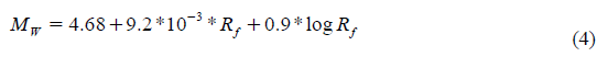
where Rf is the maximum distance, in km, from causative fault to a liquefied site, and Mw is the seismic moment magnitude.
In addition to Kuribayashi and Tatsuoka (1975), Wakamatsu (1991) have shown the relationship between magnitude, and maximum epicentral distance to a liquefied site by using 67 historic Japanese earthquakes, including 32 earthquakes which were used by Kuribayashi and Tatsuoka (1975), the equation, which has bounded with MJ>5.0, can be expressed as:
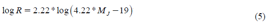
The Equation 5 has been revised, and Wakamatsu (1993) has presented a newer version of the equation to estimate the maximum range of liquefaction for specific earthquake magnitude. This relation can be given as:

where R is the farthest epicentral distance, in km, and MJ is the earthquake magnitude scale defined by Japan Meteorological Association.
Lastly, Ulusay et al. (2000) proposed the relationship between surface wave magnitude (MS) and the maximum distance R of a liquefied site for the Turkey region. Ulusay et al. (2000) have come up with an empirical formula taking the upper and the lower boundaries in consideration addition to the calculation of average value to figure out MS and R. In order to calculate a distance value (RCAL, in km), one should use focal depth and another parameter that corresponds to a distance between the projection of the epicenter to the Earth's surface and the site subjected to liquefaction. The equation can be given as follows:
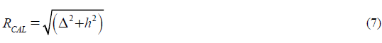
where ∆ represents the focal depth, and h stands for the projection of the earthquake source point to the Earth's surface. After that, surface wave magnitudes can be calculated by the following equations:
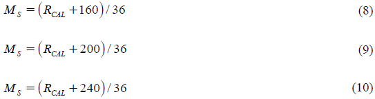
where the expression given in Equation 8 is the lower boundary for the calculation, Equation 9 and Equation 10 are the medium value and the upper boundary of the magnitude calculation, respectively. From the point of R calculation view, the same procedure is valid. In other words, Equations 11, 12, and 13 are given for R calculation (in km) with the discrimination of the upper, medium value, and the lowest boundaries, respectively.
All of these theoretical approaches were used in the maximum extent of the liquefiable area analysis part in soiLique. Merely, the medium value boundary calculation is used in the approach mentioned in Ulusay et al. (2000).
2.2. Safety Factor Analysis
The safety factor is used to understand whether the investigation area is in the safe zone against liquefaction. Various approaches have been represented by investigators to estimate the safety factor of liquefaction. The fundamental step in finding the safety factor is the division of Cyclic Resistance Ratio (CRR) and Cyclic Stress Ratio (CSR). Hence, CSR and CRR must be calculated to mention the safety factor.
CSR, which is induced by a particular earthquake, was first introduced by Seed and Idriss (1967). It is an equivalent form of the uniform shear stress, which is triggered by the corresponding earthquake (Boulanger and Idriss, 2014). Seed and Idriss (1971) has introduced
CSR with a reference value equal to 65% of the peak cyclic stress. The empirical formula of CSR is given in Equation 14:

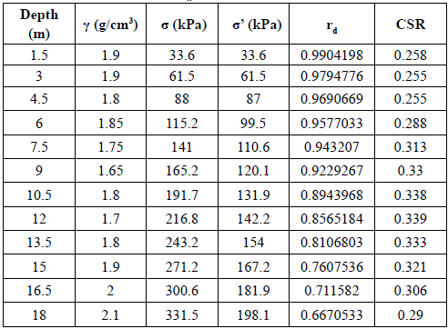
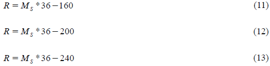
where σ0 is the total vertical overburden stress, σ0 is the effective vertical overburden stress, α max is the peak ground acceleration and r d is a stress reduction coefficient which can be calculated by:
where z is the depth of the layer in m. The calculation of stress reduction coefficient, r d , possesses other conditions for the depths of 30 m and greater. However, for cases where z is greater than 23 m, potential liquefiable layers may be neglected from the point of overburden stress view. Liquefaction assessments at greater depths frequently include specific conditions that need to be verified by detailed analyses. Because of that reason, Idriss and Boulanger (2008) have suggested completing site response studies by a high-quality site response calculations for the sites where the rd values at depths greater than approximately 20 m. That is the reason why it is used only for up to 23 m depth values in the present study.
CRR, cyclic resistance ratio, can be called the strength of the soil. Unlike CSR, CRR can be calculated from the Standard Penetration Test (SPT), Conic Penetration Test (CPT), and shear wave velocity (VS) measurements. In general, CRR curves were firstly introduced for an earthquake having a moment magnitude equals 7.5, and its symbol is CRR7.5. For different moment magnitude values, one must switch from CRR7.5 to CRR, by multiplying it with a magnitude scaling factor (MSF). It can be given as:

where Mw denotes the moment magnitude of an earthquake. Then, the safety factor, SF, can be calculated with the division of the CRR and CSR:

2.2.1. Obtaining CRR 7 from SPT Data
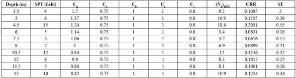
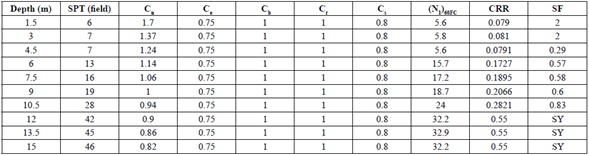
In soiLique, the methodology mentioned in Seed and Idriss (1971) is used to obtain CRR7.5. In the theory of SPT- CRR7.5 computations, SPT data must be corrected before calculations. The formulation of SPT blow count correction can be given as:

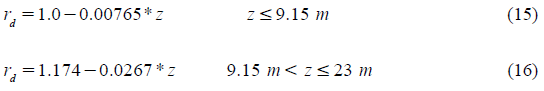
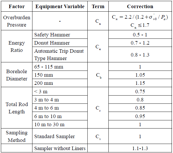
where the left-hand side of the equation represents the corrected SPT blow count, N mea is the measured SPT blow counts in a field, Cn is the depth correction factor, Ce corresponds to hammer energy ratio (ER) correction factor, C is the borehole diameter correction factor, C denotes rod length correction factor, and Cs stands for correction factor for samplers with or without liners. Details of these corrections for SPT blow count given by Youd and Idriss (2001) are also represented in Table 1.
Having the SPT N is corrected, the procedures stated in firstly Seed and Idriss (1971), and the fine content correction, which has been updated by Youd and Idriss (2001), is applied to calculate CRR7.5. The procedure starts with the formula given below:

and where α and β are:

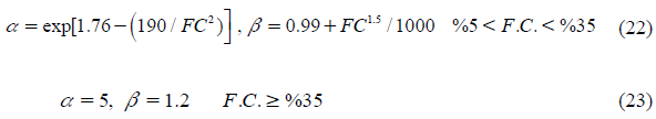
where F.C. means fine content. The Equations 21, 22, and 23 are used for calculation of the coefficients of fine content correction of SPT blow count, given in Equation 20, in terms of fines content percentage in the samples. Then, CRR7.5 can be obtained with the formula:
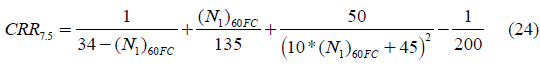
which has the upper limit at 30 for (N 1)60FC in (Youd and Idriss, 2001).
2.2.2. Obtaining CRR 7.5 from V S Measurements
Shear-wave velocities (VS) can be measured in situ with the help of several seismic techniques including cross hole, downhole, seismic cone penetrometer, suspension logger, SASW, and MASW. Their accuracy can be sensitive to processing details, soil conditions, and interpretation methods Andrus and Stokoe (2000). One can correct VS to a reference overburden stress by (Sykora, 1987; Robertson et al. 1992)

where CV = factor to correct measured shear-wave velocity for overburden pressure and can be calculated by

where VS1 is overburden stress-corrected shear-wave velocity, Pa is the reference stress of 100 kPa or about atmospheric pressure; and σ 0 is the initial effective overburden stress (kPa). Then, CRR7.5, based on VS measurements, can be calculated by;
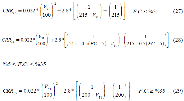
where F.C. is the representative of the fine content (Andrus and Stokoe, 2000).
2.2.3. Obtaining CRR^^from CPT Data
The CRR7.5 calculation of CPT data in soiLique is based on the technique which was published by Suzuki et al. in 1997. This technique includes the computation of a soil behavior type index, IC, and the adjustment of measured tip resistance with factor fS. This factor is also a function of the soil behavior type index. In this technique, the measured tip resistance is corrected in terms of overburden pressure with the formula given below:
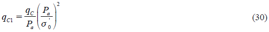
where qC1 is the corrected tip resistance, qC is the measured one, σ0 is the effective overburden stress (kPa), and Pa is the reference stress of 100 kPa or about atmospheric pressure. The next step is the calculation of the soil behavior index, which has been represented by Robertson et al. (1995) :

where Q and Rf are:
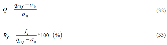
and where qc1f is the fines corrected tip resistance in tsf, fS is the measured sleeve friction, σ0 is the total vertical overburden stress, σ0 is the effective vertical overburden stress, Q is a normalized tip resistance, and Rf is a sleeve friction ratio. The last step before calculating the CRR7.5 is the adjustment of the tip resistance, and it can be achieved by the formula as follows:

qca is equivalent to the adjusted tip resistance, and as it has already mentioned before, f is the function of soil behavior index and with the range between 1 and 3.5 depending on changing values of the soil behavior type index, IC. For the values less than and equal to 1.65, f(IC) turns into one (1); and for values higher than and equal to 2.4, it takes 3.5. In the range between 1.65 and 2.4, it takes different values. In the present study, CRR 5 is calculated with the formula, which was proposed for the method of Suzuki et al. (1997), mentioned in Mollamahmutoglu and Babuccu (2006) instead of using CRR7.5 liquefaction curve versus adjusted tip resistance given by Suzuki et al. (1997).
2.3. Settlement Analysis
If the safety factor of liquefaction is known, it is possible to determine the variation of the post-liquefaction volumetric strain (Ishihara and Yoshimine, 1992). The combination of safety factor and the volumetric strain was proposed by Ishihara and Yoshimine (1992), and it is given in Figure 1.
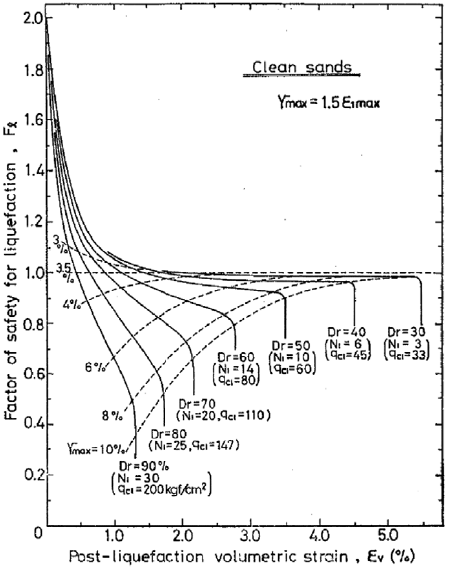
Figure 1 The combination of the safety factor, FS, and post-liquefaction volumetric strain e r (Modified from Ishihara and Yoshimine, 1992)
The relationship between corrected SPT blow count, ( N1)60, and the post-liquefaction volumetric strain was proposed by Tokimatsu and Seed (1987). The combination can be read from Figure 2.
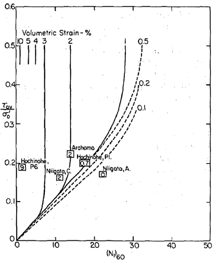
Figure 2 The relationship between corrected SPT, (N1)60, and volumetric strain (Modified from Tokimatsu and Seed, 1987)
In the present study, equations introduced by Mollamahmutoglu and Babuccu (2006) are used to compute the possible post-liquefaction settlements. They have used the curve overlaying technique and proposed equations for both methods of (Ishihara and Yoshimine, 1992) and (Tokimatsu and Seed, 1987). The objective is the computation of possible post-liquefaction settlement after the estimation of volumetric strain. Settlements can be calculated with the formula below:

where z is the thickness of the layer in m, εv is the volumetric strain, and Ssat signifies the corresponding saturated soil layer.
2.4. Simple Analysis
The relation between relative density (DR), in percentages, and peak ground acceleration (PGA), in g, has been proposed by Tezcan and Teri (1996).
According to the correlation, the intersection of DR and PGA indicates the risk of liquefaction. In this context, "risk" means the frequency of liquefaction exposure. In Figure 3, the graph of the correlation is represented; and as can be seen, three zones of different risk levels are demonstrated on it. The first one is high -risk zone, which defines if the intersection of those is located at this zone, the study area has a high risk of liquefaction. The second zone is moderate-risk, which indicates that if the intersection point of the parameters is located in this zone, the study area has a moderate risk of liquefaction. Lastly, the third one is the non-liquefiable area. If the intersection of the parameters is in that zone, the study area is out of liquefaction risk.
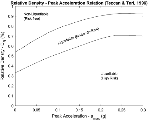
Figure 3 The graph of the relation between relative density (DR) and peak ground acceleration (PGA). Modified from Tezcan and Teri (1996).
3. Overview of soiLique
soiLique is the first MATLAB® based program with GUI that ensures deterministic liquefaction analysis with the calculation of parameters that are previously propounded with the empirical equations.
The substantial feature of MATLAB® that makes it different from other programming tools is having a matrix-based language paving the way for computation of mathematical expressions. It provides an excellent environment for any courses (Chapra, 2012). Although other environments (e.g., Excel©) or languages (e.g., C++, Fortran 90) could have been chosen, MATLAB® presently offers a combination of convenient programming features with powerful built-in algorithms (Chapra, 2012). The user-friendly nature of MATLAB® explains why it is widely used to solve scientific and engineering problems. In addition to its user-friendly nature, having rich libraries (i.e., data and image processing tools) enlarges the implementation of MATLAB®. Graphical user interface (GUI) preference permits a code writer to create an interactive program that is semi-independent of MATLAB®. Specifically, one can construct a program in GUI, set it apart from MATLAB® and then, can run it after its installation to any computer provided that the installation of proper MATLAB® Runtime Environment version. The GUI feature is the glossy point of MATLAB®, which leads to soiLique. Moreover, MATLAB® allows users to switch between other languages. For example, a code written in MATLAB® can be converted to C ++, Java, or other languages.
The algorithm presented here, soiLique, is designed for the mitigation of liquefaction triggered hazards based on four different calculation classes such as 1) SF analysis allowing estimation of SF of liquefaction with respect to shear wave velocity, SPT blow count data, and CPT data, 2) Settlement analysis that provides to evaluate calculations of settlements based on liquefaction, 3) The Evaluation of a Maximum Extent of a Liquefiable Area maintains predicting the distance of a liquefiable area to the epicenter or causative fault with corresponding earthquake magnitude, and lastly, 4) Simple analysis with only considering relative density (DR) and the peak ground acceleration (PGA) of the earthquake.
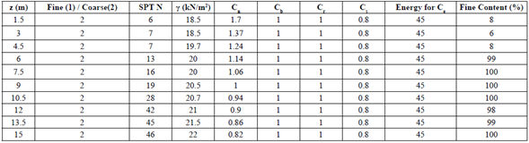
The workflow of the safety factor and settlement analyses part of soiLique is depicted in Figure 4. It can be inferred from the figure that soiLique has two main decision mechanisms. The first one is related to the specific part of the input file containing information on whether the soil structure includes fine or coarse particles. The second one is checking the shear wave velocity or SPT blow count values in both settlement and safety factor analyses.
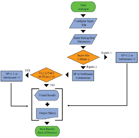
These checking mechanisms are fundamentally based on the theoretical background of the program. In order to obey the calculation rules of formulas given in the theory section, soiLique has several limitations. These limitations are listed in Table 2.
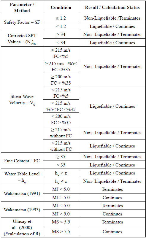
In Table 2, "terminate" means considering safety factor as 1.2 and settlement as zero for the corresponding investigation depth. In the past, some liquefaction events have been observed while SF using related methods and assumptions were calculated to be greater than 1.00. In order to be on the safe side, it would be better to consider SF as 1.2. That is the reason why SF is capped to 1.2. Of course, this does not mean that liquefaction events will not be observed definitely for values higher than 1.2. Thus, it is a threshold value for the present study, and settlements are not expected for the values higher than 1.2. In the case of SF equals to 1.2, the program supposes that the subjected layer is non-liquefiable and terminates calculations of parameters for the corresponding layer. Then it continues to calculate liquefaction analysis parameters of the next layer/investigation depth. Vs based SF analysis is designed for calculations with or without FC data. The presumption of a limiting upper value of corrected shear wave velocity, V s1 , is considered as 215 m/s for areas with F.C. less than %5, and it is the same for the areas having F.C. values between %5 and %35. The upper limit for the shear wave velocity is considered as 200 m/s for areas having F.C. values equal to and greater than %35, according to the Equation 29. This limitation is a similar presumption that is commonly made in the SPT-and CPT-based procedures dealing with clean sands, where liquefaction is considered not possible (Andrus and Stokoe, 2000). If the F.C. data is accessible besides VS measurements, one can consider it while creating the input file. In case of having no F.C. data, soiLique computes Vs based parameters based on Equation 27.
Additionally, there are several limitations to the calculation of the maximum distance of a liquefiable area, too. For instance, in the techniques of Wakamatsu (1991) and Wakamatsu (1993), the user must enter values higher than 5.0 for MJ as input. In addition to this issue, the user must recognize that soiLique only uses medium value calculations mentioned in Ulusay et al. (2000), the upper boundary and lower boundary calculations are neglected in the present study.
4. Results and Discussion
To test the robustness of soiLique, Soil Engineering, which was introduced by Ozcep (2010), was used for comparison. A real data set from Ozcep et al. (2014) is utilized in the present study for settlement and SPT-based analyses. Ozcep et al. (2014) have investigated to understand what role the soil properties play as one of the main factors causing earthquake damage in Yalova, and to compare the influence of two soil problems - amplification and liquefaction - on earthquake damage (Ozcep et al. 2014). All of the analysis sections, except settlement and SF analyses based on SPT data, were tested with synthetic data and presented under this heading.
4.1. Results of Real Data Set
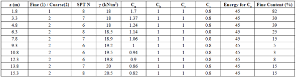
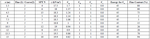
The geological characteristics of Yalova can be explained by extensive Quaternary alluvial deposits, and the Tertiary Yalakdere and Kilic formations. Borehole locations are superimposed on the geological setting map in Figure 5. The Quaternary deposits consist of stratified materials having varied grain sizes and are derived from the various geological units in the vicinity (Yilmaz and Yavuzer 2005). The main drainage system is dominated by the Samanli, Safran, Balaban, and Kazimiye rivers. Borehole records throughout the study area show that the groundwater table is generally very shallow (Yilmaz and Yavuzer, 2005; Ozcep et al. 2014).
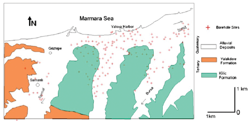
Figure 5 Map of the study region, including geological setting. Red plus signs correspond to borehole locations. Modified from Ozcep et al. (2014).
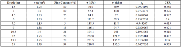
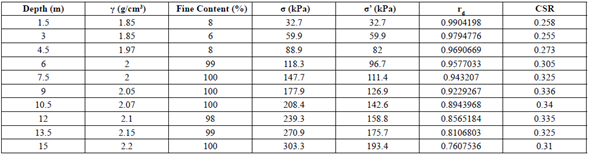
For the analysis process, the data obtained from three boreholes, BH43, BH76, and BH106, are used. Every analysis was carried out with the parameters M was considered as 7.4, and PGA was taken as 0.4 g. The water table levels ofthe boreholes, BH43, BH76, and BH106, are 2.65 m, 1.72 m, and 3.8 m, respectively. The map ofthe study area by indicating settlement distribution and locations of the selected boreholes is presented in Figure 6.
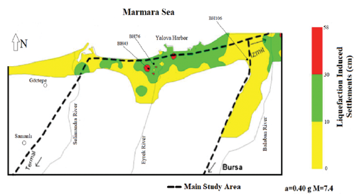
Figure 6 Map of liquefaction induced settlements of the study area using the Ishihara and Yoshimine (1992) approach. Black dots display locations of the boreholes, BH43, BH76, and BH106. Dashed lines show the boundary of the main study area. Modified from Ozcep et al. (2014).
According to the map presented in Figure 6, areas with the yellow color indicate the lowest amount of total settlement (0 - 10 cm) and, the green-colored areas correspond to middle settlement amounts (10 - 30 cm). Likewise, the red-colored areas have the highest amounts of settlement (30 - 58 cm). The selected three boreholes are relatively exemplary in terms of the amounts of different settlement quantities. The data of those boreholes were used to present a comparative study to test the robustness of soiLique.
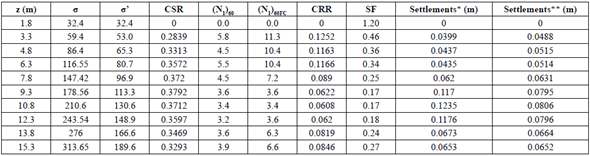
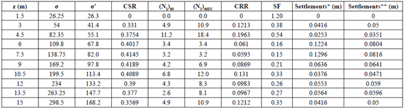
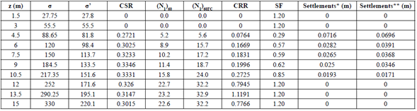
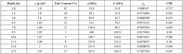
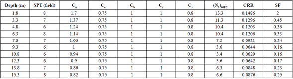
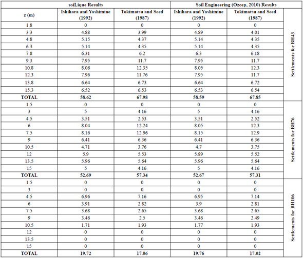
One way to compare the results can be achieved by checking how close the layer-based settlement calculations of soiLique and SoilEngineering (Ozcep, 2010) for all boreholes. The settlement amount of each layer for the borehole, BH43, can be found in Table 3. Detailed tables for the calculations can be found in the supplementary data file. Additionally, the log plots for every borehole from soiLique, and SoilEngineering (Ozcep, 2010) are presented in Figure 7, Figure 8, and Figure 9 for boreholes BH43, BH76, BH106, respectively. These figures show that trends of the variation of SF with depth are consistent. As demonstrated in Table 3, the outputs of soiLique and SoilEngineering (Ozcep, 2010) are consistent with each other. For the total settlement comparisons, the results of both software show good agreement when taking all results and plots into consideration.
Table 3 Comparison of settlement results for BH43 calculated with soiLique and SoilEngineering (Ozcep, 2010)
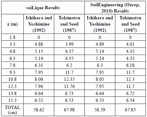
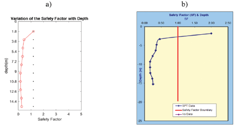
Figure 7 The variation of SF with depth for the borehole, BH43 a) from soiLique, b) from Soil Engineering (Ozcep, 2010).
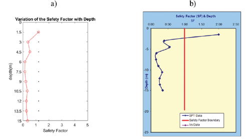
Figure 8 The variation of SF with depth for the borehole, BH76 a) from soiLique, b) from Soil Engineering (Ozcep, 2010).
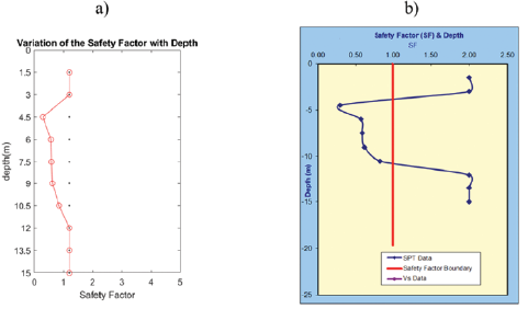
Figure 9 The variation of SF with depth for the borehole, BH106 a) from soiLique, b) from Soil Engineering (Ozcep, 2010).
The layer-based settlement graphs are presented in Figure 10. These plots are specific to soiLique. Each row in Figure 10 corresponds to the results of boreholes, BH43, BH76, and BH106, respectively. These results were obtained by using the settlement analysis based on SPT. When SF varies below the safety limit, the layer-based settlements are calculated and plotted using two different approaches, such as ones introduced by Tokimatsu and Seed (1987) and Ishihara and Yoshimine (1992). On the far left of Figure 10, panels a, d, and g, the variation of settlement for each layer plots based on Tokimatsu and Seed (1987) approach is presented. The middle panels of Figure 10, b, e, and h, the variation of settlement for each layer plots depending on the Ishihara and Yoshimine (1992) approach is demonstrated. On the far right of Figure 10, panels c, f, and i represent the relationship between CRR and SPT (N1)60 mentioned in Youd et al. (2001) is presented. soiLique represents that graph by putting a red circle where CRR and SPT (N1)60 values intersect at a corresponding layer. As can be seen from the figures, these red circles were cumulated in or around the liquefiable region. It might be evidence of consistent calculation in terms of comparison of the already proven technique.
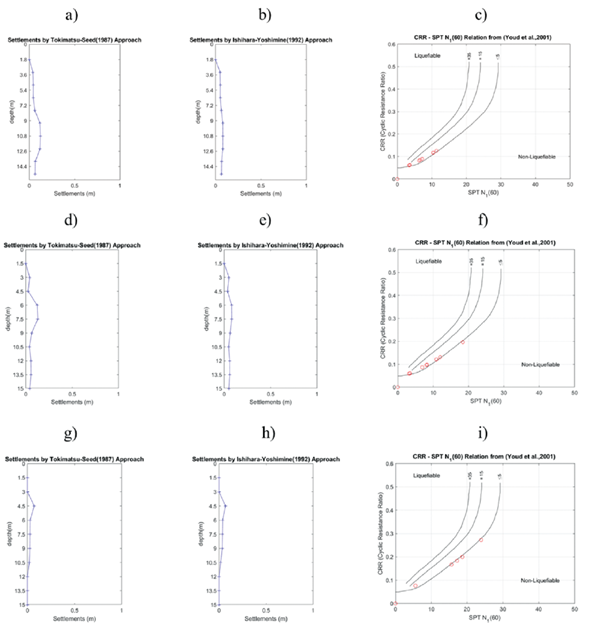
Figure 10 Other plots of results from soiLique. The first row (a, b, c) of the figure are the results for BH43 data, the second row (d, e, f) correspond to results of BH76 data, and the last row (g, h, i) shows the results of BH106 data. Panels a, d, g show the settlements for each layer with respect to Tokimatsu and Seed (1987) approach, and panels b, e, h show the settlements for each layer with respect to Ishihara and Yoshimine (1992) approach. Lastly, panels c, f, i show the CRR and (N1)60 relationship mentioned in Youd et al., (2001). This graph of relationship is digitized, and red circles correspond to CRR values.
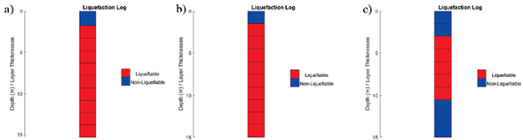
Another feature of soiLique is that plotting layer-based log plots showing liquefaction-prone layers. In Figure 11, liquefaction log plots of soiLique are demonstrated. In this figure, reds correspond to layers that are prone to liquefaction, and blues show safe layers. This kind of graphs helps the user to visualize the layers which may be prone to liquefaction. In Figure 4.7, panels from (a) to (c) are the representative of boreholes BH43, BH76, and BH106, respectively. Those logs are plotted with respect to SF values.
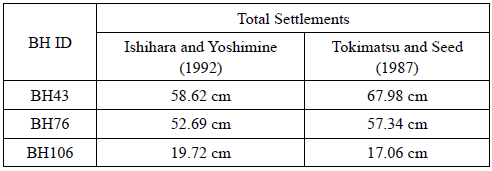
In addition to the layer-based settlement comparisons, the total settlements that were calculated by soiLique and SoilEngineering (Ozcep, 2010) were compared. A more detailed results table for the total settlement amounts is presented in the supplementary file. The total settlement amounts for every borehole calculated by soiLique, are presented in Table 4. Another way to test the robustness of the calculations done by soiLique can be achieved by using the map in Figure 6. For this testing process, the total amounts calculated by Ishihara and Yoshimine (1992) approach in Table 4 are focused only. As a result, the amounts calculated in the present study are consistent with the ranges represented in the color bar of the map. In detail, the borehole BH43 has the highest total settlement amount corresponding to the red-colored areas in Figure 6, and the borehole BH76 has the intermediate values as indicated by the green color on the map. The borehole BH106, which is located at the margin between Kilic Formation and alluvial deposits of Yalova, has the lowest total settlement amount as shown with yellow color on the map.
After pointing out the consistency between the results of soiLique and SoilEngineering (Ozcep, 2010), it would be better to mention the differences. It is obvious that small variations can be observed between the results presented in Table 3. These differences are related to the work procedures of soiLique and SoilEngineering (Ozcep, 2010). For example, soiLique assumes the highest limit for SF as 1.2, even though it is 2.0 in SoilEngineering (Ozcep, 2010). Besides, a slight difference can be observed between the results of the total vertical stress and the effective vertical stress in both software. Hence, these small differences affect CSR values. This fundamental difference occurs because soiLique considers the unit of the unit volume weight parameter as kN/m2, whereas SoilEngineering takes it as g/cm3. A comparative plot is presented in Figure 12 to show the trends of CSR and CRR values of both software. Although these differences have an impact on the calculations of the stress parameters -i.e., total vertical stress and effective vertical stress- and CSR values, it can be inferred from the figure that the mentioned differences can be neglectable. Lastly, the difference in the limitations for correction of the SPT values may cause some differences in CRR values. However, these effects are also negligible because the corresponding limits of the software are not far away from each other to affect the results negatively. These differences are valid for the VS-based calculations, which can be observed from the VS output tables in the supplementary file, and they can be neglected.
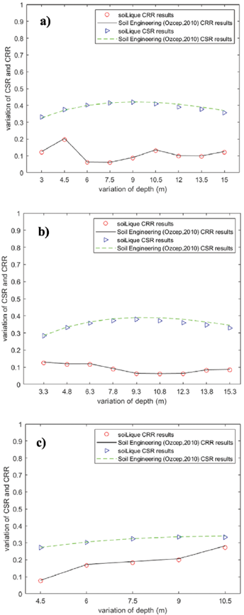
Figure 12 Comparative Plots of CRR and CSR results from soiLique and Soil Engineering for liquefiable layers of a) BH43, b) BH76, c) BH106. Red circles stand for soiLique CRR
Comparison of results from soiLique and SoilEngineering (Ozcep, 2010) reveals that although the work procedures of soiLique and SoilEngineering (Ozcep, 2010) may differ, the results are satisfactory.
4.2. Results of Synthetic Data Set
In the present study, the synthetic data set is used for showing results for safety factor analysis based on VS values and CPT data. The safety factor analysis with respect to SPT data calculations of soiLique gives the same outputs except for settlement graphs and calculations.
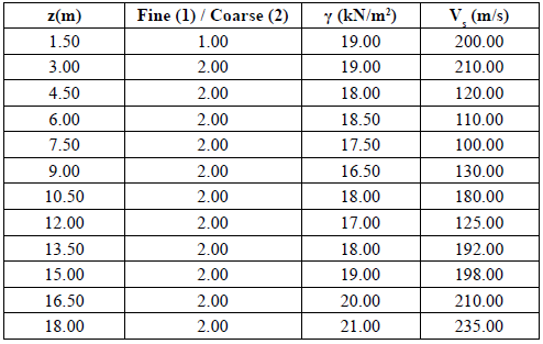
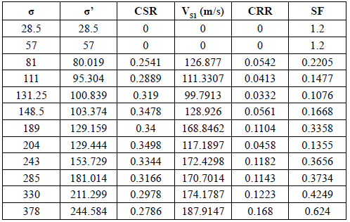
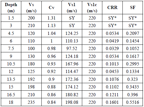
Details of the input table and result table of safety factor analysis based on Vs analysis are presented in the supplementary file. The water table level is considered as 4.4 m, M is taken as 7.4, and PGA is accepted as 0.4 g for that calculation. In Figure 13, the results of the calculation based on Vs values are presented. That type of calculation has three visual outputs. One of them is the variation of SF with depth; the others are CRR-VS1 relation, which has been represented by Andrus and Stokoe (2000), and a liquefaction log plot. The limitation of the VS based calculation is having the corrected shear wave velocities (VS) below 215 m/s; in that case, the analysis will continue. However, if the corrected Vs values are higher than 215 m/s, the corresponding layer or layers will have SF equal to 1.2. In this example, all corrected Vs values are below this limit. That is the reason why all layers have SF below 1.2.
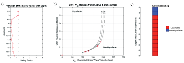
Figure 13 Outputs, from soiLique, for synthetic data that is used safety factor analysis based on VS values. a) the variation of the safety factor with depth. b) the CRR-VS1 relation that is taken from Andrus and Stokoe (2000) and redrawn with red circles at the intersection points. c) the liquefaction log. The water table level is considered as 4.4
As well as the real SPT data set, the synthetic VS data analysis is also checked with SoilEngineering (Ozcep, 2010). In this example, the fine content is not taken into consideration. Input and result tables of this analysis are demonstrated in the supplementary file. The plot of VS-based analysis from SoilEngineering (Ozcep, 2010) is shown in Figure 14. In panel a, the screenshot of CSR results for VS calculation from SoilEngineering is shown. As a comparison, both soiLique and SoilEngineering (Ozcep, 2010) consider the first two layers as not be prone to liquefaction. The trend of SF variations with depth is close to each other.
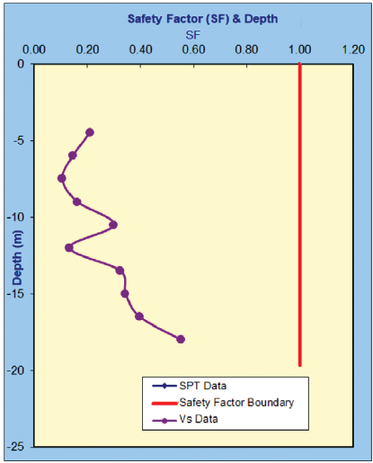
Figure 14 The graph of variation of SF with depth from SoilEngineering (Ozcep, 2010) for synthetic VS data.
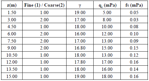
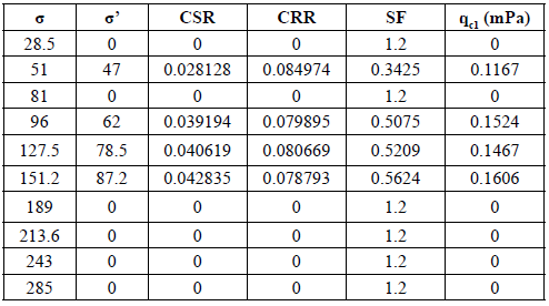
In addition to the synthetic VS data analysis, an example analysis with synthetic CPT was carried out. In this synthetic example, the water table level is considered as 2.6 m, M is taken as 7.4, and PGA is accepted as 0.4 g for that calculation. Unfortunately, the results of the CPT data set could not be compared to any other programs because a free program that performs Suzuki et al. (1997) approach cannot be found. In Figure 15, the output of SF analysis based on synthetic CPT values are displayed. The routine presented here, soiLique, gives three types of visual outputs for CPT-based analysis. One of them is the variation of the SF with respect to depth; the others are CRR - qc1 relation that has been introduced by Suzuki et al. (1997) and the liquefaction log that shows which layers are liquefiable and which are not. CRR - qc1 relation graph is redrawn after digitizing the original plot, and soiLique adds points at intersections during the calculation.
In the second graph of Figure 15, one can observe that most of the red circles were gathered in the liquefiable region. These layers are responsive ones to liquefaction. That plot is one of the evidence for the calculation accuracy of soiLique.
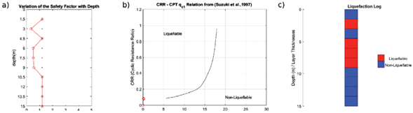
Figure 15 Outputs, from soiLique, for synthetic data that is used safety factor analysis based on CPT values. a) variation of the safety factor with depth. b) CRR - qc1 relation is taken from Suzuki et al. (1997) and redrawn with red circles at the intersection points. c) liquefaction log. The water table level is considered as 2.6 m, MW=7.4, and PGA= 0.4 g.
A simple analysis can be carried out by using soiLique. In the presented algorithm, the output is a graph that is replotted from Tezcan and Teri (1996) with a red plus at the intersection point of those two parameters. For example, in this study, DR is considered as 0.6 (%), and PGA is taken as 0.25 g to represent a plot. As a result, if the study area possesses DR and PGA as or similar to those taken in that example, it means that the corresponding area has a substantial risk of liquefaction. The output of this example can be found in the supplementary file.
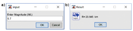
Lastly, the maximum extent of a liquefiable area was carried out as an example. The output can be found in the supplementary file. The theory mentioned in Liu and Xie (1985) is used to calculate the maximum extent of a liquefiable area during an earthquake with ML equals 6.7. As a result, the maximum extent is 23.945 km.
5. Conclusion
We have presented the first deterministic liquefaction analysis GUI written in MATLAB®. The capability of soiLique for performing liquefaction analysis is presented through two separate data sets, real and synthetic data. In order to check the robustness of soiLique, results were compared with another program, SoilEngineering (Ozcep, 2010). In terms of work procedure, soiLique and SoilEngineering (Ozcep, 2010) differs from each other.
Although SoilEngineering (Ozcep, 2010) has multiple calculation sections for a wide range of geotechnical problems, soiLique is focused only on deterministic liquefaction analyses. Moreover, soiLique includes alternative approaches for the calculation of the maximum extent of a liquefiable area, although SoilEngineering (Ozcep, 2010) includes only one of them. Likewise, soiLique provides to visualize the boreholes in terms of liquefaction.
The results demonstrate that soiLique obeys the limitations during calculations. For example, the choice of fine or coarse option in the second column of the input file directly affects the calculations as expected. In this study, the limitations of soiLique are presented in Table 3.1. As can be seen from the table, soil layers with SPT values greater than 34, and in most cases, the shear wave velocity greater than 215 m/s is accepted as non-liquifiable by soiLique. The limitation for F.C. is 35%, meaning that layers having F.C. lower than 35% is liquifiable. Additionally, it is evident that the limitations for Fine Content, SPT blow counts, VS values, and the CPT-based calculations affect the results properly.
Comparisons were made to check whether the results of soiLique and SoilEngineering (Ozcep, 2010) are consistent or not. These tests reveal that results were satisfactory and coincident with each other. That is to say; the calculated total settlement results yield a good agreement with the results of the previous study and SoilEngineering (Ozcep, 2010). The key features ofsoiLique are its easy-to-use nature, and being equipped with a variety of deterministic liquefaction analyses. In addition to these, its specific visual results make it easier to understand the liquefaction phenomenon for users. Consequently, soiLique is proven useful in terms of determination of the liquefaction triggered settlements and SF with short computation time.
6. Code Availability
soiLique is available as an open-source code and can be downloaded from the web site [https://github.com/ekrembkn/soiLique]. In the same directory, a user guide and examples can be found. It can be redistributed and/or modified under the terms of GNU Library General Public License 3.0. The user can download "soiLique.exe" to use it without MATLAB® instead of source codes, optionally.