


 English (pdf)
 Article in xml format
 Article references
 Send this article by e-mail
 Cited by SciELO
  Cited by Google
  Similars in
SciELO
Similars in
SciELO  Similars in Google
 Permalink
Introduction
Global Navigation Satellite Systems (GNSS) have been commonly used for positioning for decades. However, the positioning accuracy obtained by the GNSS is prone to error sources, which can be primarily categorized as clock-related errors, signal propagation errors, system errors, and intentional errors (selective availability and signal jamming etc.) (Karaim et al., 2018). The quality of the obtained positioning accuracy is expressed with two metrics. The first metric is the user equivalent range error (UERE) that defines the total errors on the pseudorange. The range between satellites and the receiver is called the pseudorange due to the noise and errors. The second quality metric is the dilution of precision (DOP) that specifies the effect of geometry on the relationship between positioning and measurement (Chen et al., 2013; Li et al., 2018; Teng et al., 2015; Teng & Wang, 2016). Accurate positioning can be obtained with the good spatial spread of the visible satellites that provide lower DOP values (Banerjee & Bose, 1996; Verma et al., 2019). DOP is utilized for the optimum selection of visible satellites (Teng & Wang, 2014) and is categorized as the horizontal dilution of precision (HDOP), vertical dilution of precision (VDOP), and time dilution of precision (TDOP). The combination of HDOP and VDOP is named position dilution of precision (PDOP), and the variety of PDOP and TDOP is called the geometric dilution of precision (GDOP).
Global Positioning System (GPS) is still the most reliable satellite-based positioning system designed to have at least six satellites at any part of the Earth (Busznyák et al., 2019; Wang et al., 2011). However, in some environments such as urban areas, heavy tree cover, open-pit mines, etc., the desirable number of GPS signals cannot reach the receiver due to the signal blockage by obstacles (Alkan et al., 2015). In this case, a weak or no positioning solution can be obtained. In the last decades, multi-GNSS solutions have been investigated to exceed this limitation and acquire more accurate and reliable positioning results (Alkan et al., 2017). In the last years, multi-constellation solutions have been worked with GPS/GLONASS, GPS/BEIDOU, GPS/GALILEO, GPS/GLONASS/BEIDOU, GPS/GLONASS/GALILEO, and GPS/GLONASS/GALILEO/BEIDOU in many studies. The multi-constellation positioning ensures improved positioning solutions using more visible satellites with better geometric distribution and more satellite availability (Wang et al., 2019).
The tropospheric and ionospheric errors are the two primary error sources related to signal propagation. The seasonal changes of atmospheric variables like temperature, water vapour, hydrostatic pressure, and humidity significantly affect these errors. The effect of seasonal variation on the GNSS accuracy was analyzed by Dogan et al. (2014). They concluded that the GNSS positioning accuracy in summer is better than that in winter. Additionally, Saracoglu & Sanli (2020) studied the effect of seasonal changes on GNSS positioning in different world regions. They concluded that the seasonal impact on positioning accuracy changes according to climate zones. In Zheng et al. (2018), zenith tropospheric delay accuracy was investigated on the GNSS data. The results showed that the accuracy in winter is better than in the other seasons. Many seasonal atmospheric factors affect GNSS signals quality and positioning. Therefore, the results of the seasonal effects on GNSS positioning accuracy differ from the others.
The analysis of the GNSS measurements is critical in geodesy due to working conditions in the field. Some experiments can be performed, and the results can be investigated to shorten the working time in the field. In the process of obtaining measurements, a lot of factors affect the GNSS measurements. The experimental design methods can be used frequently to determine the significant factors on the response variable. The primary and interactive effects of dependent variables (x) can be determined using the experimental design process on the response variable (y). The statistical analysis and graphical presentation make the interpretation of the results easier. Also, a suitable experimental design model will reduce the required data and spend time on the field (Çoruh et al., 2012; Seltman, 2018).
There are different experimental designs such as Full Factorial, Plackett-Burman, Tagucci Box-Behnken design, and central composite design (Gündogdu et al., 2016). Full factorial design (FFD) is a widely used procedure to determine dependent variables' primary and interactive effect on the response variable in different levels, such as 2p, 2p-k, 3p (George et al., 2005; Navidi, 2008; Sisman, 2014a).
The experimental design has been used in many engineering applications. Geomatics engineering uses many types of application data from different sources for positioning. The size of application data has increased a lot in recent years, and therefore the analysis of application data has become more critical. Experimental design is one of the analyzing methods of application data, but the experimental design is limited in geomatics. The main aim of this study is to investigate the factorial effects of the season, the number of satellites, and DOP on the CORS horizontal and vertical positioning errors using FFD. Although there are some studies in geodesy that have investigated the factor effects on the GNSS positioning (Abad & Suárez, 2004; Ahmad, 2015; Brenneman et al., 2010; Cai & Gao, 2007; Catania et al., 2020; Pirti, 2008; Raghunath et al., 2011; Stone & Powell, 1998; Svabensky & Weigel, 2004; Wielgosz et al., 2019; Wing et al., 2008; Yoshimura & Hasegawa, 2003), there is no study in literature for network-real-time-kinematic (NRTK) using FFD. The factorial effects at two levels were studied using a 23 FFD in this study. The regression equation as y = f(x) was obtained from the NRTK horizontal and vertical positioning error results.
The rest of this paper is organized as follows. In section 2, GNSS positioning and the factorial design are explained in detail. The results and discussions are presented in Section 3. Finally, the conclusions are given in Section 4.
Material and Methods
GNSS Positioning
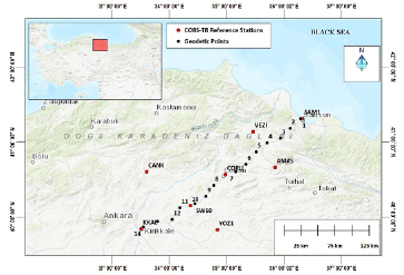
This study was conducted along a 280 km long route from Samsun to the Kirikkale provinces of Turkey. Fourteen geodetic points were established with 20 km intervals through the course. The locations of geodetic points and the stations of the Continuously Operating Reference Stations Network of Turkey (called CORS-TR or TUSAGA-AKTIF) around the geodetic points are shown in Figure 1.
TUSAGA-Aktif delivers real-time GNSS correction data to the receivers of NRTK systems 24/7 like the other countries. TUSAGA-Aktif system was established with 146 reference stations using baselines ranging 70-100 km across Turkey and Northern Cyprus (Aykut et al., 2015; Gülal et al., 2013). This system transmits the correction data with Virtual Reference Stations (VRS), Flachen Korrectur Parameter (FKP), and Master Auxiliary Concept (MAC) techniques in GSM, Networked Transport of RTCM via Internet Protocol (NTRIP), and radio connections by Radio Technical Commission for Maritime Services (RTCM) 3.0 and higher protocol (Bakici et al., 2017). The obtained 3D coordinates are in the International Terrestrial Reference Frame 1996 (ITRF96) datum and 2005.0 epoch with cm-level accuracy (Ilçi, 2019).
A Trimble R10 GNSS receiver for GNSS observations was used. The site surveys were conducted in two different periods (winter and summer) to determine the seasonal effect on GNSS measurement accuracies. In winter, the site surveys were conducted on two consecutive days (December 1st and 2nd, 2017), and site surveys in summer were executed on June 2nd and 3rd, 2018. The GNSS receiver was mounted on the geodetic points to determine the reference position of the sites in the winter and summer periods. (Soler et al., 2006) revealed that 2-hour static sessions are sufficient to obtain the desired accuracy for 280 km baseline length between the base and the rover stations. (Firuzabadi & King, 2012) obtained mm level horizontal and vertical precisions where the baseline lengths were less than 200 km in 2 hours. In this study, taking into account the baseline lengths between 1 to 100 kilometres and the open sky area conditions, we determined the GNSS static observation duration as 100 minutes. Simultaneously, the receiver was connected to the TUSAGA-Aktif service and the CORS data were collected for 10 minutes with 1-second intervals, and the elevation mask was set to 10 degrees. Although the TUSAGA-Aktif service only transmits the correction data related to GPS and GLONASS constellations, we have observed all GPS, GLONASS, GALILEO, BEIDOU, and QZSS constellations at all geodetic points for further analyses.
2.2 Factorial Design
The factorial design investigates the effect of two or more factor levels on the response variable using designed experiments. Thus, the mathematical model can be obtained between the main and interactive effects of factors and response variables; also, the time, effort, and operational cost can be reduced (George et al., 2005; Ismail et al., 2008; Montgomery, 2001; Navidi, 2008). If the factors have a main or interactive effect on the response variable in the experimental design, their results can be determined as significant. Although there are several factorial design methods, the 2p FFD is the most preferred method. 2 and p show different levels and the number of factors, respectively (Box et al., 2005; Gygi et al., 2006; Ismail et al., 2008; Wu & Hamada, 2009).
The two aims were realized by FFD. One of them is mathematical model development between selected factors and response variables. This mathematical model is a regression equation, including main and interactive effects, given in Equation (1).

Here; β 0 , β i , and β ij are the main and interactive effects' coefficients; and are the factors; e is the error of the mathematical model. The second aim of FFD is to test significance of factors on the obtained mathematical model. In this stage, the null and alternative hypotheses are established. The main and interactive effects of factors are tested according to the selected significance level using the analysis of variance (ANOVA). More details of FFD can be found in (George et al., 2005; Gygi et al., 2006; Montgomery, 2001; Navidi, 2008).
Results and Discussion
In this study, the season, number of satellites, and DOP data were taken as factors; the CORS's horizontal and vertical positioning errors were taken as a response variable, and 23 FFD was established. The level of factors was taken as high (+1) and low (-1). The levels of the season, satellite number and DOP were selected for summer as (high) and for winter as (low); >15 (high) and <15 (low); <1.4 (high) and >1.4 (low), respectively. The high (+1) and low (-1) levels of factors are shown in Table 1.
Table 1 The levels of factors.
| Factor | Low Level (-1) | High Level (+1) |
|---|---|---|
| Season (X1) | Winter | Summer |
| Satellite Number (X2) | <15 | >15 |
| DOP (X3) | >1.4 | <1.4 |
The design matrix of application data was taken from the data obtained from CORS-TR as explained in Section 2.1 (Table 2). Minitab 16 statistical software was used for all the analyses of the experimental process (Minitab, 2021).
Table 2 The design matrix of application data.
| Run No. | Factor | RMS | |||||
|---|---|---|---|---|---|---|---|
| X1 | X2 | X3 | Horizontal Errors (mm) | Vertical Errors (mm) | |||
| 1st Trial | 2nd Trial | 1st Trial | 2nd Trial | ||||
| 1 | Winter | <15 | >1.4 | 15.2 | 15.3 | 20.6 | 20.8 |
| 2 | Summer | <15 | >1.4 | 10.1 | 10.2 | 16.5 | 16.7 |
| 3 | Winter | >15 | >1.4 | 9.11 | 9.6 | 14.3 | 14.6 |
| 4 | Summer | >15 | >1.4 | 10.4 | 11.0 | 17.0 | 17.9 |
| 5 | Winter | <15 | <1.4 | 10.1 | 10.3 | 15.3 | 15.7 |
| 6 | Summer | <15 | <1.4 | 10.3 | 10.5 | 15.8 | 17.5 |
| 7 | Winter | >15 | <1.4 | 10.5 | 11.1 | 16. 3 | 17.8 |
| 8 | Summer | >15 | <1.4 | 9.2 | 9.9 | 15.0 | 16.0 |
The descriptive statistic is a supply to understand the data by users using central tendency (mean, median, mode, quartiles) or variability (range variance, skewness, etc.) (Sharma, 2019). There are several graphical methods to represent the descriptive statistic parameters (Potter, 2006). The box plot analysis of application data was realized (Table 3 and Fig. 2).
Table 3 Results of the descriptive statistical analysis of application data.
| Application Data | Mean (mm) | St.Dev. (mm) | Mínimum (mm) | Median (mm) | Maximum (mm) |
|---|---|---|---|---|---|
| Horizontal Errors | 10.8 | 1.8 | 9.1 | 10.3 | 15.3 |
| Vertical Errors | 16.7 | 1.9 | 14.3 | 16.4 | 20.8 |
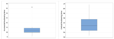
Figure 2 The box plot of application data. The box plot represents that the min, max, Q1 (%25), Q2 (median), Q3 (75%) and mean values of application data.
Firstly, the mathematical model was obtained for the application data (Table 4). The significance of factors was determined using a hypothesis test. If the P-value of the factor is bigger than the significance value (selected as %5 in this study), it is decided that the factor is insignificant in the regression model.
Table 4 Estimated effects and coefficients for CORS horizontal (left) and vertical (right) positioning errors.
| Term | Effect | Coef. | P-Value | Term | Effect | Coef. | P-Value |
|---|---|---|---|---|---|---|---|
| Constant | 10.8110 | 0.000 | Constant | 16.740 | 0.000 | ||
| X1 | -1.2030 | -0.6015 | 0.000 | X1 | -0.392 | -0.196 | 0.288 |
| X2 | -1.4069 | -0.7035 | 0.000 | X2 | -1.259 | -0.629 | 0.006 |
| X3 | -1.1158 | -0.5579 | 0.000 | X3 | -1.140 | -0.570 | 0.011 |
| X1*X2 | 1.2480 | 0.6240 | 0.000 | X1*X2 | 1.097 | 0.549 | 0.013 |
| X1*X3 | 0.7005 | 0.3502 | 0.002 | X1*X3 | 0.175 | 0.087 | 0.625 |
| X2*X3 | 1.2840 | 0.6420 | 0.000 | X2*X3 | 1.483 | 0.742 | 0.003 |
| X1*X2*X3 | -1.9609 | -0.9804 | 0.000 | X1*X2*X3 | -2.436 | -1.218 | 0.000 |
| S=0.299 | R-sq=98.56% | S=0.688 | R-sq=92.91% | ||||
In Table 4, Coef. and P-values, S and R-sq represent the regression equation coefficient, the student-test value of factors, standard deviation and the ratio of explained variation to total variation, respectively. It was seen that all main and interactive factors except X1 and X1*X3 on the vertical positioning had a significant effect on the response variable. In this case, the insignificant term should be removed, and the regression coefficient determined with substantial factors. The regression equation of the response variable, for horizontal and vertical positioning, is given according to Equations 2 and 3, respectively.
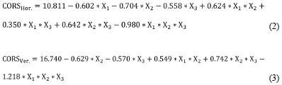
The response variable can be increased or decreased according to the multiplication of coefficients and the levels of factors. Since the CORSta and CORSver. are supposed to decrease; this multiplication is desired to have a negative sign.
In this study, the main effects should have negative signs in Equation 2 and Equation 3. Therefore, the level factors can be taken as (+1) for equations 2 and 3 for the main effects. On the other hand, the interactive effects of factors should be considered. According to the magnitude of coefficients in Equation 2, since the coefficients of X1*X2 and X2*X3 are bigger than X1 and X3 coefficients and the coefficient of X1*X2*X3 are the maxima the X1, X2, and X3 should be taken as (-1), (+1) and (-1). Also, according to the magnitude of coefficients in Equation 3, since the coefficients of X2*X3 is bigger than X2 and X3 coefficients and the coefficient of X1*X2*X3 is the maximum, the X1, X2, and X3 should be taken as (-1), (+1) and (-1).
The R2 is the rate of explained variability and total variability and describes the goodness of fit for the model (Mason et al., 2003; Seltman, 2018; Sisman, 2014b). In this study, R2 was equal to 98.56% and 92.91% for the CORS horizontal and vertical positioning errors, respectively. This means that 98.56% and 92.91% of the application data can be explained with the obtained mathematical model.
Moreover, the ANOVA test is realized in the FFD. The ANOVA results of horizontal and vertical CORS positioning errors were obtained for application data (Table 5). It is decided that the effect has a significant impact on the response variable if the P-value is more powerful than the selected significance value (5%).
Table 5 ANOVA for horizontal (left) and vertical (right) CORS positioning.
| Source | DF | Adj SS | Adj MS | P-Value | Source | DF | Adj SS | Adj MS | P-Value |
|---|---|---|---|---|---|---|---|---|---|
| X1 | 1 | 5.7893 | 5.7893 | 0.000 | X1 | 1 | 0.6132 | 0.6132 | 0.288 |
| X2 | 1 | 7.9177 | 7.9177 | 0.000 | X2 | 1 | 6.3372 | 6.3372 | 0.006 |
| X3 | 1 | 4.9800 | 4.9800 | 0.000 | X3 | 1 | 5.1951 | 5.1951 | 0.011 |
| X1*X2 | 1 | 6.2300 | 6.2300 | 0.000 | X1*X2 | 1 | 4.8155 | 4.8155 | 0.013 |
| X1*X3 | 1 | 1.9627 | 1.9627 | 0.002 | X1*X3 | 1 | 0.1225 | 0.1225 | 0.625 |
| X2*X3 | 1 | 6.5947 | 6.5947 | 0.000 | X2*X3 | 1 | 8.7977 | 8.7977 | 0.003 |
| X1*X2*X3 | 1 | 15.3799 | 15.3799 | 0.000 | X1*X2*X3 | 1 | 23.7319 | 23.7319 | 0.000 |
In table 5, DF, Adj SS, Adj MS, P-Value represent the degrees of freedom, adjusted sums of squares, adjusted mean squares, the fisher-test value of factors, respectively. Some graphical representations such as the Normal Plot of the Standardized Effects can also obtain the effects of factors on the response variable. The normal probability plots are used to estimate the significance of interaction effects in a factorial design (Kavuri et al., 2009). The magnitude, direction, and importance of the effects can be determined using the normal probability plot of the effects. Figure 3 illustrates the Normal Plot for application data.
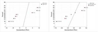
If the effects are close to the distribution fit line, they have no significant impact on the response variable. It was also seen that although all main and interactive results were significant on the CORS horizontal positioning error, the X1 and X1*X3 effects were not significant on the CORS vertical positioning error. The change effect of the factor level can be seen with the main effect plots. The main effect plots are given in Figure 4.
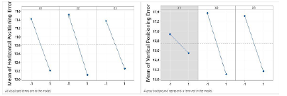
It was determined that the (+1) level of all factors had reduced the horizontal and vertical CORS positioning errors. Also, it was seen that the X1 (i.e. the seasonal effect) was not a significant effect on the response variable of the vertical component. Since the effects have a high slope, it is decided that selecting factor levels is suitable for this study.
The interactive effect of the factor level can be obtained from Interaction Plot. For this study, the interaction plots were given in Figure 5.
It was seen that while only the X1*X3 interaction does not have a significant effect on the CORS vertical positioning error, the other interaction effects were substantial in both the CORS horizontal and vertical positioning errors. If the 2-effect factor levels have the same slope, it will not be meaningful on the result variable. The main results of the study can be summurazed as follows;
R2 values were satisfactory (98.56% for CORS horizontal, 92.91% for CORS vertical positioning errors).
All main and interactive effects of factors were significant on CORS horizontal positioning errors at the 5% level.
Season (X1) and Season*DOP (X1*X3) effects of factors were insignificant on CORS vertical positioning errors at the 5% level.
The 3-way interaction effect Season*Satellite Number*DOP(X1*X2*X3) had the most significant coefficient on the regression models of CORS horizontal and vertical positioning errors.
Conclusions
This study aimed to investigate the effects of factors on CORS positioning using statistical design experiments. For this, a 23 full-factorial design (three factors at two levels) was established to evaluate the main and interaction effects of season, the number of satellites, and DOP on the CORS positioning. The main conclusions for the study are shown below:
The minimum values of CORS horizontal and vertical positioning errors were 9.1 mm and 14.3 mm in the case of the winter season, bigger than 15 satellite numbers, and bigger than 1.4 DOP, respectively.
The maximum values of CORS horizontal and vertical positioning errors were 15.3 mm and 20.8 mm, in the case of the winter season, lower than 15 satellite numbers, and bigger than 1.4 DOP, respectively.
The factors levels should be taken as (+1) levels (Summer, >15, and < 1.4) considering the main effects of factors. But it is seen that when the interactive effects were added to the regression model, the factors should be taken as (-1) levels for Season and DOP, (+1) level for the number of satellites.
The value of CORShor. was calculated 9.6 mm with (+1) levels (Summer, >15 and <1.4) of factors. But the value of CORShor. was calculated 9.4 mm with (-1) levels (Winter and >1.4) of seasons and DOP and (+1) level (>15) of the number of satellites because of the interactive effects of factors on the response variable.
While the value of CORSver. is calculated 15.6 mm (+1) levels (Summer, >15 and <1.4) of factors. But the value of CORShor. was calculated 14.1 mm with (-1) levels (Winter and >1.4) of seasons and DOP and (+1) level (>15) of the number of satellites.
In the light of these explanations, it can be said that the main and interactive effect of the number of satellites was always (+1) levels (>15); the other factor levels (seasons and DOP) can be changed for application data.
Many different application data sources must be analyzed attentively in applied sciences such as geomatics engineering. It is seen that the experimental design is quite helpful and practical for positioning applications, as it demonstrates the factor effects on positioning error. The statistical analysis and graphical presentation of the experimental setup are easier to understand the application data. Also, the regression equations derived from the experimental design allow investigating different levels of selected factors on the CORShor. and CORSver. easily. It is suggested that the experimental design studies must be carried out in other areas of geomatic engineering such as remote sensing, photogrammetry and surveying.

