


 English (pdf)
 Article in xml format
 Article references
 Send this article by e-mail
 Cited by SciELO
  Cited by Google
  Similars in
SciELO
Similars in
SciELO  Similars in Google
 Permalink
Introduction
The rainfall - runoff relationship in a watershed involves a set of physical and chemical processes which intervene at different spatial and temporal scales (Plesca et al., 2012; Ocampo et al., 2014;), and in turn, the watershed is influenced by weather conditions, soil properties, land use and topographic characteristics (Marín et al., 2014; Martínez et al., 2017).
However, the scarce information in the Andean watershed is a limitation in order to analyze these relationships, which is why hydrological models have been implemented, as a key tool to understand the runoff generation, provide hydrological forecast and therefore, contribute to the planning and management of hydrological resources. (Chen et al., 2020; Plesca et al., 2012).
One of the widely used models is the CN curve number method was developed in 1972 by the Soil Conservation Service (SCS) of the U.S. Department of Agriculture (USDA) as a simple application methodology for calculating runoff in a rainfall event and whose criterion does not require the study watersheds to be gauged or instrumented (Aparicio Mijares, 1992; Chow et al., 1994; Ibáñez-Castillo et al., 2014; Pérez Nieto et al., 2015).
In the SCS-CN model, the generated runoff is obtained from the recorded rainfall, the initial abstractions or losses (considered as 20% of maximum soil retention) and curve number (CN), which is obtained from tables designed according to soil type, land use, conservation practices in agricultural areas, and hydrological condition (Chow et al., 1994; Ibáñez-Castillo et al., 2014).
According to Ibáñez-Castillo et al. (2014) and Montiel Gonzaga et al. (2019), the SCS-CN model is one of the most used techniques in the hydrological field due to its simplicity and medium information requirement (Pacheco Moya, Quiala Ortiz, & Martinez Hernandez, 2018), even it is one of the methods used by Soil and Water Assessment Tool (SWAT) model to predict runoff (Neitsch et al., 2011).
Nevertheless, the model has been subject to several critical revisions by authors as Hawkins (1993), Ponce & Hawkins (1996), Lopez (2001), Mishra et al. (2007) y Paz-Pellat (2009). That is how Hawkins (1993) stated that it is difficult to accurately select the appropriate CN from the tables and that the runoff calculation is much more sensitive to the chosen CN than to the rainfalls presented because rainfall records are more closely tracked, while the CN values are unique to the area studied or analyzed and are only found in the tables developed by the SCS.
In view of the foregoing, Hawkins (1993) proposed to use the SCS-CN model in an inverse way to calculate CN. In order to do this, Hawkins solved the mathematical equations for the SCS-CN for model (Eq. 1-2) and let rainfall and runoff as model variables (Eq. 7). In this way, it is possible to calculate CN with the rainfall and runoff data in a watershed. However, this methodology shows that there is not a unique CN value for a watershed, but a secondary relationship emerges between CN and the rainfall, giving rise to a graph which characterizes the type of response pattern of the watershed and is classified as "complacent", "violent" or "standard", the latter being the most common scenario (Hawkins, 1993).
The evaluation proposed by Hawkins (1993) have been implemented in different parts of the world which had runoff observed data as USA (Hawkins, 1993; Durán-Barroso et al., 2016; Santikari & Murdoch, 2019), Argentina (Ares, Varni, et al., 2012), Mexico (Ibáñez-Castillo et al., 2014; Pérez Nieto et al., 2015), Brasil (da Cunha et al., 2019; Durán-Barroso et al., 2016) India (Gundalia & Dholakia, 2014; Lal et al., 2015, 2017, 2019) and South Korea (Ajmal et al., 2015); in all these studies a great diference between the CN of SCS-CN model and the CN derived from observed data was found, showing that SCS-CN method cannot calculate runoff properly.
In addition, other deficiencies and limitations in the model have been considered, Ponce & Hawkins (1996) mentioned that the method does not take into account the spatial and temporal variability of infiltration and other losses by abstractions. In this regard, Merz & Bárdossy (1998) said that spatial variability might have a strong influence in the runoff- rainfall relationship. Likewise, López (2001) stated that calculation methodology does not take into account the effects of rainfall intensity, it means, that for the calculation carried out in two selected events, with the same rainfall but of different duration, the runoff will be the same.
In the case of tropical conditions, no evaluation studies of the SCS-CN model have been found, but the scientific evidence presented here highlights the importance of evaluating the SCS-CN model, where the frequency of intense rainfall has increased, its records show high spatio-temporal variability on low scales, and in addition, temporal information is scarce (Marín et al., 2014).
In Colombia, the SCS-CN model is widely used to calculate runoff, mainly due to the easy implementation of the model. However, the absence of flow monitoring stations (CVC, 2015) has been an impediment to the validation of the SCS-CN model, therefore, it is not really known whether the model works properly under tropical conditions. Then, the current investigation aims at evaluating the Curve Number model (CN) under conditions of a tropical Andean micro watershed using the methodology proposed by Hawkins (1993).
Materials and Methods
Micro watershed Study: Description of La Vega
La Vega micro watershed is located in the municipality of Palmira, Valle del Cauca, Colombia; its drainage area is immersed in the Aguaclara sub watershed, which is the main tributary of the Bolo River.
The study area comprises 3°30'33.12'' to 3°29'53.52'' North and 76° 10' 54.48'' to 76°11'44.52'' West, with an extension of 114.08ha, an altitudinal range of 1400 to 1900 m.a.s.l. an average slope of 21% and average multi-annual monthly rainfall of 1800 mm.
The average multi-annual monthly rainfall in the area presents a bimodal regime, with two wet periods in the months of March-May and October-December, as well as two periods of less rainfall in the months of January-February and June-September.
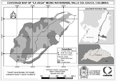
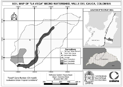
Groundcover in the micro watershed (Fig. 1) are permanent shrub crops (coffee crops) (53%), cultivated grass (34%), shrubs and bushes (13%). Soils (Fig. 2) are Typic Dystrudepts (85%) and Typic Humudepts (7%), which are characterized by being deep, well drained, with fine textures, medium to low organic carbon content in depth and low moisture retention; meanwhile, Typic Udorthents soils (8%) are superficial, limited by the presence of rock fragments, moderately well drained and low moisture retention (CVC; IGAC, 2014).
Rainfall and flow measurement
The study micro watershed kept a detailed record of rainfall and flow with a time resolution of 15 minutes. The information was collected from June 2015 to July 2017 by the Centro de Investigación de la Caña de Azúcar de Colombia - CENICAÑA.
Rainfalls in La Vega were recorded using a Davis Vantage pro-2 weather station located into the micro watershed at an altitude of 1607 m. Flow monitoring was performed continuously at the micro watershed hydrometric station, consisting of a water level sensor (through a Keller brand Acculevel pressure sensor), installed in a narrow crest weir to ensure a control section and accurate flow measurement.
Runoff calculation with SCS-CN Method
The SCS-CN method presents runoff as a function of rainfall (daily rainfall or 24-hour rainfall) and soil water storage capacity, calculated by the expression:
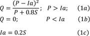
Where P is the rainfall in mm; is the initial abstraction of the watershed in mm; Q is the runoff generated in mm and S is the maximum soil retention in mm, the latter related to CN by:
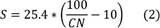
The CN was obtained from tables according to soil type, land use, conservation practices in agricultural areas, and hydrological condition (Chow et al., 1994; Neitsch et al., 2011b; Ibáñez-Castillo et al., 2014). For this purpose, information was obtained from the semi-detailed soil survey at a scale of 1:25000 (Fig. 1) of the watersheds prioritized by the environmental authority of the department: Corporación Autonoma Regional del Valle del Cauca (CVC) (CVC; IGAC, 2014); in the same way, information on land use was obtained (Fig. 2), which was validated and compared with information collected in field visits.
To select the hydrological soil group, the four groups of soils described by Chow et al. (1994) were taken into account, these groups are presented in Table 1, also in this table can be observed the soil type associated with the hydrological soil group.
Table 1 Hydrological soil group
| Soil Groups | Description | La Vega soils |
|---|---|---|
| Group A | Deep sand, deep soils deposited by the wind, aggregated silts | - |
| Group B | Shallow deep soil deposited by the wind, sandy loam | Typic Udorthents |
| Group C | Clay loams, shallow Sandy loam, soils low in organic content, and soils usually high in clay | Typic Dystrudepts and Typic Humudepts |
| Group D | Soils that swell significantly when wet, heavy plastic clays, and certain saline soils. | - |
Source: Adapted from Chow et al. (1994)
Once the hydrological soil group for each soil type was found, the CN was determined for the different land uses in the micro watershed according to the CN tables presented by Neitsch et al. (2011b). In order to obtain an average CN for the hole watershed, CN was weighted by area using ArcGIS 10.4.1 following the methodology proposed by Chow et al. (1994).
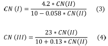
The selected CN was corrected for antecedent humidity (Eq. 3,4) and slope (Eq. 5) (Ibáñez-Castillo et al., 2014; Pérez Nieto et al., 2015); in terms of humidity, there are three types of CN classified according to previous rainfall (during the 5 days prior to the runoff event), to determine the adjustment. Thus, CN data recorded in tables by the SCS are assumed in normal antecedent moisture condition (AMC II) (Chow et al., 1994). Criteria for defining the antecedent moisture condition are presented in Table 2.
Table 2 Antecedent Moisture Condition Classification
| AMC group | Total 5-days antecedent rainfall (mm) | |
|---|---|---|
| Dormant season | Growing season | |
| I | ≤ 13 | ≤ 36 |
| II | 13 - 28 | 36 - 53 |
| III | ≥ 28 | ≥ 53 |
Source: Adapted from (Ferrer Polo, 2000)
For the correction for antecedent moisture (Table 2), the growing station was selected, since in both periods of the bimodal regime there are rainfall records of significant magnitude. Calculation for equivalent CN is presented in Equations 3-4.
The slope correction (Eq. 5) was introduced because CN tables proposed by the SCS were developed for use in watersheds with slopes of less than 5% (Nash & Sutcliffe, 1970):
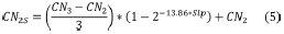
Where is the curve number corrected for slope; is the curve number for the AMC (III) group; is the curve number as read in the SCS tables; Slp is the mean slope of the watershed (m/m). In this study, the CN derived from SCS tables and adjusted by slope and moisture will be termed CNAMC2S
Runoff Calculation from Observed Flow (Baseline Method J + N)
To determinate actual runoff in the micro watershed, 55 rainfall events and its flow responses were analyzed during June 2015 and July 2017. These 55 events were considered because presented a clear flow response as a result of a single rainfall event. These clear flow response events were easily identified in the hydrograph by an ascent curve (Qa), a single peak flow (Qmax) and finally a descent curve (Qd). In the present study, only events of a single peak were considered and were referred to as unique events. Figure 3 represents a typical case of a unique event presented in the study area. Different kinds of flow responses were not considered because runoff cannot be calculated by the Baseline Method J + N.
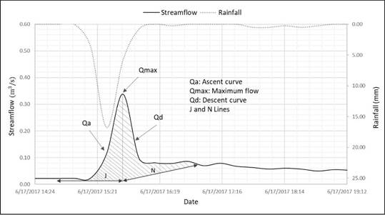
The start of the event was determined when the level sensor showed a significant increase in river flow as a consequence of rainfall; this start was projected horizontally until the moment of peak on the hydrograph (J) and ended with a diagonal according to the fixed base flow method (Chow et al., 1994), where it is assumed that runoff ends in a fixed time N (Eq. 6) in the recession segment.
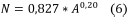
Where N is the number of days after the peak on the hydrograph, and A corresponds to the watershed area, given in Km2. Figure 3 graphically explains this method.
The event initial flow was determined as an average for flows recorded two hours prior to the start of the event; runoff was calculated as the area under the hydrograph curve and delimited below by the J and N lines (inclined); runoff (mm) was calculated by dividing the total runoff volume by the micro watershed area.
Influence of rainfall intensity on runoff generation
To evaluate the influence of precipitation intensity in runoff generation, the methodology proposed by Wischmeier y Smith (1978) to determine maximum 30 minutes precipitation intensity (I30) in an erosive event was used. This methodology is considered into the erosivity factor of the Universal Soil Loss Equation (USLE). I30 values were obtained for the 55 analyzed events and were related with observed runoff (Baseline Method J+N).
Determination of the observed CN (CN q )
To determine actual CN (CNQ) an inverse SCS-CN modeling was performed (Hawkins, 1993). For that, each of the 55 actual rainfall events data and its runoff responses (calculated by J + N methodology) were introduced in Equation 7.
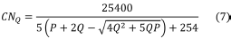
The Equation 7 results from solving the maximum retention of the soil (S) in Equation 1a and substituting this value in Equation 2. 2.6 Estimation of Adjustment between CN AMC2S and CN q
To measure the level of adjustment between CNAMC2S and CNQ, the Nash efficiency index (E) was used (Nash & Sutcliffe, 1970), which has been widely used in the evaluation of hydrological models (Yusop, Chan, & Katimon, 2007; Pérez Nieto et al., 2015), calculated from the following equation:
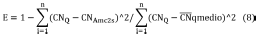
The Nash efficiency index can have values from -∞ to 1; when the Nash index is closer to 1, hydrological model prediction (in this case SCS-CN) is better.
Asymptotic Adjustment Method
To determine the type of response pattern of the studied micro watershed, the rainfall and runoff values measured in the watershed (55 unique events summarized in section 2.4) were ordered independently and in descending order, subsequently the CN values were determined for each pair of data (rainfall and runoff) using the Equation 7 then, the relationship between rainfall and CN was plotted. According to Hawkins (1993), three types of patterns can occur in this rainfall-CN relationship: "standard", "violent" and "complacent" behavior.
In cases of responses patterns "standard" or "violent", the CNs approach a constant value with increasing rainfall, and these are given by the Equations 9-10 respectively.
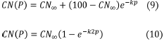
Where is a constant value approached as and is a fitting constant (different for each behavior).The variable describes the data set for larger rainfall events (Hawkins, 1993).
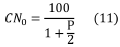
In the "complacent" behavior, evidences no appreciable tendency to achieve a stable CN value (Hawkins, 1993). Deeper mathematical analyses of Equations 1-2 were developed, where the effects of the variables Ia and S were shown to be minimal; thus, the CN was rethought as a rainfall-dependent variable (Eq. 11) and was considered the lower limit of the curve number definition (Hawkins, 1973).
Results and Discussion
In the 55 unique events analyzed in the micro watershed, the maximum recorded rainfall was 74 mm and the minimum was 0.3 mm, while the antecedent moisture (five previous days) varied from 0 to 105 mm.
SCS-CN method
CN values obtained from SCS tables
The CN values were calculated by tables according to SCS method. Due to micro watershed heterogeneity (soil and land use), there were several CN values for the micro watershed. Table 3 presents the CN weighted by area for "La Vega" micro watershed, its slope correction (CN2s), and its antecedent humidity correction (CNAMC2S).
Table 3 CN found by the SCS methodology.
| Weighted | CNAMC2S | ||||
|---|---|---|---|---|---|
| Micro watershed | CN | CN2s | CN I | CN II | CN III |
| La Vega | 73 | 76.8 | 58.2 | 76.8 | 88.7 |
Runoff Calculated from CN tables (CN AMÍC2í )
The runoff SCS-CN method calculated from CN tables was 2.3 mm on average, with a maximum value of 39.6 mm and a minimum of zero; in Figure 4, lines present the runoff calculated from CN tables (CNAMC2S) with respect to rainfall in the La Vega micro watershed in its three humidity conditions (CN I, CN II, CN III) (Feyereisen et al., 2008). The points represent 55 events studied in the micro watershed and the runoff generation according to the SCS-CN model.
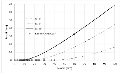
Figure 4 Evaluation of runoff (CNAMC2S) - rainfall relationship in La Vega, according to the SCS-CN model.
Figure 4, shows that 42 events out of the 55 analyzed correspond to low antecedent moisture (CN I line), it means most of the CN data were below the "mean condition" (CN II) defined by the SCS, just 5 events corresponded to CN II condition and 8 to CN III condition
It is important to note that SCS-CN model is strongly influenced by the antecedent moisture because the correction of the CN from the antecedent humidity affects in an inverse way Ia (as described in equations 1 and 2) and, consequently, in the generation of runoff.
To show the humidity correction effect, similar rainfall events recorded in the micro watershed (low: 15mm and high: 70mm) were taken under the three antecedent moisture conditions, which are presented in Table 4.
Table 4 Example of Some Rainfall Events
| Differences in rainfall | Date (dd/mm/yyyy) | Pp (mm) | Antecedent. Moisture (mm) | Antecedent. Moisture condition (AMC) | CN AMC2S | Initial abstractions Ia (0.2*S) | Runoff (mm) |
|---|---|---|---|---|---|---|---|
| 30/09/2016 | 69.3 | 13.2 | I | 58.2 | 36.54 | 5.0 | |
| High rainfall | 13/09/2016 | 74.4 | 37.1 | II | 76.8 | 15.35 | 25.7 |
| 13/03/2017 | 67.8 | 105.2 | III | 88.4 | 6.67 | 39.6 | |
| Low rainfall | 07/05/2017 | 15.0 | 20.8 | I | 58.2 | 36.54 | 0.0 |
| 08/05/2017 | 15.5 | 35.8 | II | 76.8 | 15.35 | 0.0 | |
| 10/05/2017 | 13.7 | 56.9 | III | 88.4 | 6.67 | 1.2 |
In this table, it can be observed that rainfalls close to 70 mm (High rainfall) presented very different runoffs (from 5 to 39.6mm), this was due to the fact that from condition I to condition II the CN changes 32%, but the impact in runoff calculated by the model was 414%. From condition I to condition III the impact was even stronger, with a CN change of 52%, runoff increases by 692%. In low rainfall, records around 15mm were taken. For this case, the impact was not so strong. All this indicates that the impact of the antecedent moisture condition becomes stronger in high rainfall.
Runoff Calculation from Observed Flow (Baseline Method J + N)
Runoff calculated from observed flow (J+N baseline methodology) had lower result than runoff of SCS-CN methodology. Runoff average value was 0.6 mm with a maximum of 6.5 mm and a minimum of zero.
In Figure 5 the three antecedent moisture curves were plotted (as shown in Fig. 4) and over this data was plotted the relation between rainfall and runoff calculated from observed flow (J+N baseline methodology) as black dots. Here, it can be observed that the runoff calculated from J+N methodology (runoff J+N) presented a trend toward the CNI curve set forth in the SCS-CN model; likewise, its values were lower than those obtained in the SCS- CN methodology. For this reason, no points were observed in the CNII and CNIII lines despite the fact that runoffs in both methodologies were calculated from the same rainfall events observed in the micro watershed.
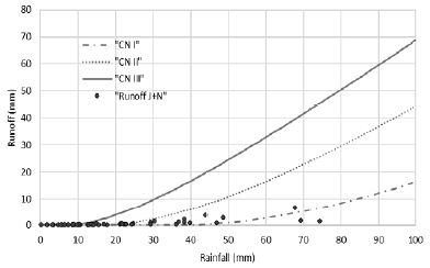
Figure 5 Evaluation of the runoff (J+N) - rainfall relationship in "la Vega", according to the SCS-CN model.
Similar results were found by López (2001), who conducted a literature review where he stated that runoffs less than 12.7 mm (half an inch) make the SCS-CN method less accurate. On the other hand, studies from Ares et al. (2012) and da Cunha et al. (2019) found that events in hydrological condition III overestimated modelled runoff.
Based on this, it can be deduced that the CNAMC2S selected from tables, corrected for slope and antecedent humidity, would be overestimating the micro watershed runoff. In addition, rainfall events where found the SCS-CN model assume runoff as (zero), while the observed data reported runoff. In cases of low runoff, the limit imposed by the SCS-CN model (P> = Ia) based on the relationship between Ia and S (X = 0.20 in equation 1c) may not be adequate. This agrees with authors such as Ajmal et al. (2015) and Lal et al. (2015, 2017, 2019) who stated that the optimized initial abstraction ratio (X) values showed that the original assumption of the X of 0.20 is unusually high.
Influence of rainfall intensity on runoff generation
When evaluating the influence of the intensity of rainfall on the generation of runoff, the results showed that there is a clearer relationship between maximum rainfall intensity and runoff (R2 = 0.96) than between amount of rainfall and runoff (R2 = 0.42) (Fig. 6). Since the runoff process is the result of the interaction of the rainfall rates (intensity) and the infiltration rate, it makes more sense to use the rainfall intensity as a variable in the model instead of the amount of rainfall as expressed by Santikari & Murdoch (2019), who consider that taking temporary variations into account can improve the performance of the SCS-CN model.
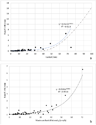
However, it is more complex to measure intensity than amount of rainfall, especially at the time the SCS-CN model was implemented but now with the current development of automatic stations, it may be feasible to incorporate rainfall intensity in runoff calculation.
CN derived from runoff' (CNQ
The CNq was calculated using the SCS-CN model in an inverse way (Eq. 7), which already had the influence of slope and antecedent moisture, due to the fact that its calculation was made from real runoff data in the micro watershed
For the 55 unique events of the micro watershed, the corresponding CNQ were found; their values oscillated between 48 and 99 with a mean of 80, indicating that most of the CNq found were high (>70) unlike the CNAMC2S which showed a tendency of 58.2 (CNI). In addition, each event had a different CNQ value and it was not possible to classify them in unique values of CNI, CNII, CNIII as in the case for CNAMC2S.
Similarly, the Nash efficiency index (Nash & Sutcliffe, 1970) was -3.04, indicating that there was no similarity between the values of CNAMC2S and CNq, therefore, the two CN were not comparable, even though both start from the same model (Eq. 1 - 2) proposed by the SCS. In this case, by finding a Nash efficiency of less than 0 it can be inferred that the CNq is a better predictor than CNAMC2S (Yusop et al., 2007; Pérez Nieto et al., 2015)
Ares et al. (2012) stated that the variety of CNq values could initially be related to the heterogeneity of soils and micro watershed coverages and secondly, to the antecedent moisture of each event. However, in the Figure 7 it can be evidenced that, unlike CNAMC2S which is stratified by the antecedent moisture (three horizontal lines), the CNq was not influenced by this factor (white triangles), for example, for an antecedent moisture of 18 mm, the CNQ varies between values of 62 and 96 (Fig. 7a).
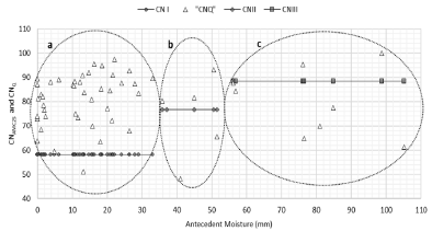
Figure 7 CNAMC2S (black circles, rhombus and squares) and CNq (white triangles) variation with respect to antecedent moisture condition (AMC) in La Vega. a. AMC I. b. AMC II. c. AMC III.
Thus, it was deduced that the antecedent moisture correction proposed in the SCS-CN methodology is a parameter that does not work properly in the actual micro watershed conditions. As mentioned in the previous section, it is possible that other aspects have a great impact on runoff, such as rainfall distribution and intensity which is not considered by SCS-CN model.
3.4 Standard Asymptotic Adjustment
To identify the micro watershed response type, the CNQ values found were related to the recorded rainfall, as proposed by Hawkins (1993), giving rise to the graph presented in Figure 8. Further, CN0 (Eq. 11) was calculated and was found that it is always lower than the CNQ (Eq. 7), which allowed to verify that variable Ia was actually a runoff lower limit as suggested by the model.
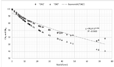
Figure 8 showed an inverse proportional relationship between the CNQ and the rainfall recorded, as the latter increases, the CNQ tends to decrease. This allow to conclude that there is a clear relationship between the CNQ and the recorded rainfall, as it was expected.
Although, this relationship did not reach a stable CNQ value, thus coinciding with the "complacent behavior" type response pattern (Hawkins, 1993), whose definition suggests that micro watershed of the present study did not respond in accordance with Equation 1a, at least not within the range of the analyzed data.
In these cases, Hawkins (1993) stated that it was possible to fit the equation for the standard behaviour (Eq. 9) with the least squares method, assuming that the data set is merely the lower rainfall end of the standard behavior pattern, and that the watershed will perform in the extrapolated standard pattern when these larger storms are eventually encountered.
Therefore, the "Standard asymptotic adjustment method" was used, obtaining the following adjustment =0.95):

In Equation 12, a CN∞ of 44.62 was defined for high rainfall events and it describes the CNq trend in the case of rainfall events of significant magnitude, however it is a much lower CN value than those analyzed in the set of data presented in Figure 8 (Hawkins, 1993).
According to Figure 8, events with rainfalls between 20 to 50 mm were related to a CN between 60 to 80, and rainfall lower than 20 mm with a CN greater than 80, the latter being the most frequent events in the micro watershed studied here. According to Hawkins (1993), values such as those observed at the beginning of Figure 8, are due to the fact that low rainfall with low CN do not generate significant runoff.
Similar results were found by Ares et al. (2012), in the Videla stream watershed, they found a "standard" category response pattern (Hawkins, 1993), and thus obtained a single CN of 57 for large events in their study area. Ares et al. (2012) had similar rainfalls in the analyzed events compared to our data (0-120mm), although Ares et al. (2012) average events were longer (69h) than the average events analyzed here (20h).
Data presented here showed that CNAMC2S presents a direct relationship with the antecedent moisture condition (Fig. 7), however, the relationship between AMC-CNQ was null; on the other hand, the variation of the CNQ obtained from observed data (Fig. 8) might be attributed to the effect of the intensity rainfall in the generation of runoff, evidenced in Figure 6a; thus, the intensity runoff could be the object of study in future investigations of the SCS-CN model.
Conclusions
The estimation of the adjustment between the curve numbers obtained from the table and those calculated from the observed runoff (CNAMC2S and CNq) showed a high diference between these values (E=-3.04), indicating that SCS-CN method does not calculated runoff properly in La Vega micro-watershed.
According to the calculations made for the runoff estimation, it was found that the CN-SCS model overestimates the runoff generated in the micro watershed, nevertheless, in some rainfall events where the SCS-CN model assume no runoff (zero), the observed data reported runoff, this was related to the limit imposed by the SCS-CN model (P> = Ia) based on the relationship between Ia and S (X = 0.20) which may not be adequate.
The SCS-CN model is strongly influenced by the antecedent moisture correction; however, according to observed data (CNQ), the AMC does not work properly in "La Vega" micro watershed real conditions.
A CN-rainfall relationship emerges when CNs are calculated from rainfall-runoff data observed (CNQ), although this relation is not considered into de SCS-CN model. Thus, the variation of the CNq in the micro watershed might be attributed to the fact that the intensity rainfall is not taken into account in the SCS-CN model.
In "La Vega" micro watershed a clear relationship between maximum rainfall intensity and runoff (R2 = 0.96) was found. This relationship is not considered in SCS-CN model. Thus, taking rainfall intensity into account in future investigations, can improve the performance of the SCS-CN model.
This study highlights the importance of assessing the applicability and limitations of the models that were developed a long time ago (such as the SCS-CN model) and which are still widely used without the knowledge of the real impact of being applied in different conditions of its development, in this case, tropical conditions.

