


 Inglés (pdf)
 Articulo en XML
 Referencias del artículo
 Enviar articulo por email
 Citado por SciELO
  Citado por Google
  Similares en
SciELO
Similares en
SciELO  Similares en Google
 Permalink
Introduction
Detachment and transportation of soil particles by overland flow are the most important causes of land degradation in water erosion-prone environments (Ollobarren et al., 2016). Dilferent stages of linear erosion development, such as rilling and gullying, irreversibly affect the health and resilience of soil systems (Su et al., 2010; Chaplot et al., 2005). Gullies are defined as deep channels formed by accumulated overland flows that multiple mechanisms, such as cutting, penetration, and tension gap progression, encourage their development. These erosional landforms commonly develop on hillslope due to the simultaneous effects of multiple geo-environmental variables, including land cover, land use, lithology, topography, soil type, and climate (Gayen et al., 2019).
Soil degradation induced by water erosion is the most critical challenge faced by many of the world's dryland regions, such as Iran. Iran is recognized as the second in the world in terms of soil erosion where approximately 2.5 billion tons of fertile lands are lost per year. Gully erosion can stimulate multiple environmental hazards, such as desertification, increasing sediment load in rivers and reservoirs, flood, and soil productivity loss (Fox et al., 2016; Ekholm and Lehtoranta, 2012). Although this hazard occurs on a small scale, its consequences will have a substantial impact on global scales. For example, gully erosion with disturbing the condition of sequestration and decomposition of soil organic carbon encourages instability in the atmospheric carbon dioxide concentrations and influences climate change (Xiao et al., 2017; Yigini and Panagos, 2016). To minimize this hazard and the related environmental problems, it is necessary to understand mechanisms controlling gully development. Furthermore, determining the magnitude and spatial distribution of erosion susceptibility zones can help to implement geo-conservation and management efforts for mitigating disasters associated with this hazard.
The gully erosion susceptibility assessment is the first step towards geo-conservation and restoration efforts in gully-prone areas (Conoscenti et al., 2014). Multiple quantitative and qualitative models have been proposed to estimate this hazard, such as the Limburg Soil Erosion model, Universal Soil Loss Equation, European Soil Erosion model, Chemical Runoff and Erosion for Agricultural Management System, Water Erosion Prediction Project model, bivariate statistical models, and logistic regression. These models could not consider the interactions among factors controlling gully erosion, such as topographic variables, geo-environmental factors, soil conditions, land use/ cover, sediment yield, and climatic indices. Compared to bivariate and logistic regression models, machine learning algorithms are the ideal models to assess erosion susceptibility, which efficiently predict the probability of gullying with high accuracy (Micheletti et al., 2014). To date, some studies have predicted potential erosion-prone areas in watersheds using these models. Chen et al., (2021) predicted the gully erosion within a watershed located in Iran using boosting ensemble machine learning algorithms. Lei et al., (2020) evaluated gully erosion susceptibility in a catchment located in Iran using four data mining techniques, including random forest, credal decision trees, kernel logistic regression, and best-first decision tree. Arabameri et al., (2020) mapped erosion susceptibility by applying four models of support vector machine, artificial neural network, general linear, and maximum entropy in the Golestan Dam basin, Iran. Saha et al., (2020) delineated the areas with the most severe gully erosion susceptibility using the algorithms of tree ensemble, random forest, and gradient boosted regression tree. Pourghasemi et al., (2020) assessed the efficacy of multiple machine learning algorithms to predict gully erosion occurrence. Amiri et al., (2019) evaluated the importance of factors controlling gully development within a watershed and mapped its susceptibility using machine learning algorithms. Gayen et al., (2019) produced a gully erosion susceptibility map in the Pathro catchment, India using different machine learning algorithms. Garosi et al., (2019) compared the reliability and discrimination of four machine learning models to map gully erosion susceptibility in western Iran.
In the present study, the importance of conditioning factors in gully erosion occurrence was assessed using the Boruta algorithm, as a feature selection algorithm that acts independently from the predictive models of gully erosion to determine the most important factors, while previous studies selected the most important causative factors based on the derivatives of the employed models. In the next step, the evidential belief function model was employed to evaluate the relationship between gullied locations and conditioning factors. Finally, considering the importance of this hazard and its global consequences, the present study employed predictive machine learning techniques, including support vector machine with two kernel types and boosted regression tree for modeling the occurrence of gully erosion within a prone watershed located in northern Iran. Finally, the predictive performance of the models was evaluated in terms of their discrimination and reliability.
Materials and Methods
Study region
The present study was implemented on Gorganrud watershed located in Golestan province, northern Iran (37"30'00" to 37"50'00"N and 55"31'40" to 56"02'10"E) (Figure 1). The maximum and minimum altitude of the watershed is 2,180 and 46 meters above sea level. Based on the Iranian Meteorological Organization, the study area's climate is semi-arid with an average annual temperature of 18.2 °C and 385 mm mean annual precipitation. More than half of the region exhibits mountainous morphology belonging to the Alborz Mountains, with a slope between 0-61°. Figure 4 illustrates the most important characteristics of the study region in terms of land use/cover and lithological structure. Rangeland is the dominant pattern of land use in the study region. In addition, loess deposits are the main deposits over the region. Based on the soil taxonomy system, the soil type of the studied region is classified under the Mollisol order. These factors caused that over 70% of the region suffered from various degrees of soil erosion as multiple rills and gullies. Mean annual soil losses caused by the gully erosion in the region estimate approximately 160 tons per hectare. The watershed area in the upslope parts of the rill and gully sites is variable between 2,000-43,070 m2. This condition strongly affected the rate of runoff discharge into rill channels, encouraging the accelerated progression of the channels (Figure 2).
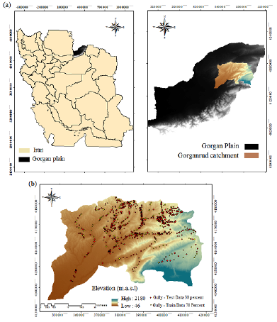
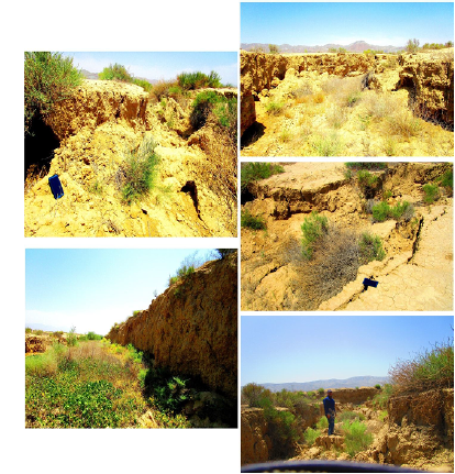
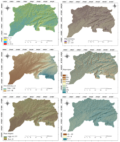
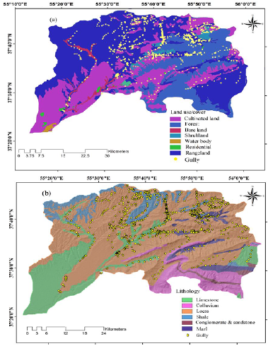
Figure 4 Spatial distributions of gullied locations in different types of land use (a) and lithological units (b)
2.2 Methodology
The methodology employed in the present study includes the following steps: after the generation of the gully inventory map, information on twelve factors controlling gully development was prepared. In the next step, the spatial correlation among gullied locations and causative variables was determined using the evidential belief function algorithm (EBF). The importance of causative factors was then weighed using the Boruta algorithm. In the final steps, the spatial prediction of gully erosion susceptibility was modeled using the support vector machine (SVM) model with two kernel types (linear kernel and radial basis function) and boosted regression tree (BRT) algorithm. The predictive performance of models was discriminated using the receiver operating characteristic curve (ROC) and the area under the curve (AUC). The reliability of model accuracy was also evaluated using the coefficient of determination (R2, for the calibration) and root mean square error (RMSE).
Gully inventory map
The first step for the modeling process is preparing the gully inventory map, exhibiting the spatial distribution of gullied locations within the study watershed. Considering the present and historical distributions of gullies, the future risk of the gully development can be predicted. Based on data taken from the Natural Resources Organization of Golestan province, gullied locations were determined. Then, these data were validated through field surveys and Google Earth images. Overall, 1,041 gullied areas were mapped in the study region. To split the gully data into two datasets of validation (30%) and train (70%), a randomly partitioned algorithm was employed using the Sub-set Features Tools in ArcGIS (Figure 1b).
Gully conditioning factors
Gully erosion is a threshold-dependent process, which different conditioning factors stimulate the occurrence and development of this hazard (Gayen et al., 2019). To predict gully erosion, using different machine learning models, the identification of factors affecting gully development is an important step. Based on previous studies (Zabihi et al., 2018; Arabameri et al., 2018) and field survey, twelve conditioning factors were considered as independent variables affecting erosion.
These variables included elevation, slope gradient, slope aspect, topographic wetness index (TWI), stream power index (SPI), plan curvature, drainage density, distance from the river, distance from the road, distance from the fault, lithology, and land use/cover.
The most important topographic factors that affect gully erosion are the elevation and slope gradient (Conoscenti et al., 2014). These factors significantly control vegetation density, climatic conditions, surface runoff, and drainage intensity. The slope aspect is another factor that plays a crucial role in the gully erosion process. This factor regulates the drying effect of winds, morphological structure of the watershed, and rate of rainfall, and related runoff, which in turn, influences the occurrence of gully erosion (Gayen et al., 2019). The erosive power of overland flows can be illustrated by the stream power index (Eq. 1), which considers contributing area and slope. The soil moisture conditions within different slope positions can be evaluated by topographic wetness index (Eq. 2). Change in this index affects the erosive power of overland flow. The convexity and concavity of a watershed are determined by plan curvature (i.e. different watershed positions), which influences gullying.
All the terrain variables were extracted from the 20 m ASTER DEM. SPI and TWI were calculated as (Bell et al., 1995; Moore et al., 1993):
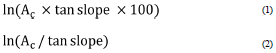
where Ac is the upslope area that drains through a certain point per unit contour length, which is equal to a certain grid cell width (Radula et al.,2018).
The occurrence of gully erosion is most probable along the fault, river, and road due to erosion and ground instability. Therefore, the maps of drainage density, distance from rivers, faults, and roads were prepared using a 1:25,000-scale topographical map. The map of drainage density was generated in ArcGIS (Line Density tools). The maps of distance from fault, river, and road were generated using the Euclidean distance function in ArcGIS. The lithology map was produced based on the geological maps on a scale of 1:50,000. The land use/cover was mapped by using Landsat 8 satellite and Google Earth images. Figure 3 and Table 2 show the classification of all the conditioning factors.
Analysis of multi-collinearity among independent variables
The multi-collinearity analysis represents the linear correlation among the measured independent variables. A very high correlation among factors encourages multi-collinearity. To determine the multi-collinearity of the factors, the variance inflation factor (VIF) and tolerance (TOL) were employed. The VIF greater than 5 and TOL less than 0.2 represent a high correlation between the variables. Since these high correlations reduce the accuracy of the results, factors with this characteristic should be removed from the final analysis. The following equations represent the calculation of VIF and TOL.
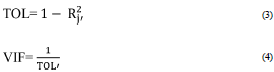
where represents the regression value of jon other variables.
Assessment of correlation between independent variables and gullied locations
The EBF algorithm was employed to assess the relationship between the independent variables and gullied locations. This algorithm is based on the Dempster-Shafer theory (Dempster, 1967; Shafer, 1976), which evaluates the uncertainty sources affecting the occurrence probability. This statistical model includes the degree of disbelief (Dis), the degree of belief (Bel), the degree of plausibility (Pls), and the degree of uncertainty (Unc) (Althuwaynee et al., 2014). The Pls and Bel were defined as the lower and upper limits of probabilities. The uncertainty degree (Unc) determines based on Bel - Pls. Dis illustrates the degree of disbelief based on 1 - Unc - Bel or 1- Pls. The sum of Unc, Dis, and Bel is calculated as 1 (Lee et al., 2012; Carranza et al., 2005). Further information on this algorithm can be seen in the research of Park (2011).
Evaluation of the importance of independent variables
The selection of variables that have the most importance in gully erosion is a crucial step in the modeling process. The importance of the independent variables controlling gully erosion was determined by applying the Brouta algorithm. Boruta algorithm is a variable selection algorithm. It is a wrapper algorithm around Random Forest (Liaw and Wiener, 2002). When a dataset comprised of multiple variables is given for modeling, this algorithm can determine the most important conditioning variables.
Machine learning models for predicting gully erosion
The Support vector machine model was initially presented as a supervised learning technique (binary classifier) that can consider linearly multi-dimensional and non-separable datasets (Kalantar et al., 2017; Kavzoglu et al., 2013). This model generates functions from a training dataset and can distinguish classes in high-dimensional feature space. In the present study, the factors controlling gully erosion (as different thematic layers) are considered as the high-dimensional feature spaces. Then, the optimal hyper-plane maximizes the margin to split into two classes, including non- gullying and gullying. The optimal hyper-plane was computed based on the equations below.
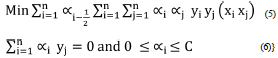
Where is the penalty factor; represents Lagrange multipliers. Regarding the present study, as a vector of input space includes factors controlling gully erosion. The non-gullied and gullied pixels were determined as +1 and -1, respectively.
This model decreases the possibility of over-fitting error and linearity and, therefore, has high efficiency to process data with nonlinear interactions by the kernel function (Naghibi et al., 2015). This algorithm has several kernel types to measure the errors that can significantly influence the prediction performance of the model and the result accuracy. The most important kernel functions of the SVM are: polynomial kernel, sigmoid kernel, radial basis, and linear kernel. This study compared the efficiency of the radial basis function (RBF-SVM) (Eq. 7) and linear kernel (LN-SVM) (Eq. 8) for modeling the gully erosion susceptibility.
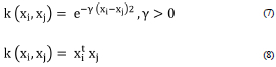
where y, d, and r are defined as kernel width, polynomial degree, and parameter of the kernel functions, respectively (Pradhan, 2013).
Boosted regression tree model (Eq. 9) adaptively combined machine learning techniques to produce an appropriate performance (Elith et al., 2008). BRT combines different regression algorithms and boosting builds to reduce the final model variance and enhance predictive accuracy (Aertsen et al., 2010). This model, with large volume of inputs, stimulated the speed in data processing and, subsequently reduced sensitivity to over-fitting.

where , m, and are defined as a classification function with a parameters and x variables, the stage of the model, and the weighting factor m, respectively.
To process the models, the spatial correlation among conditioning variables and gullied locations was first calculated. In the next step, the data was transformed into the R statistical software. Finally, the maps of gully erosion susceptibility were generated in the ArcGIS software based on the outputs of the models. The susceptibility maps were classified into five categories, including low, very low, moderate, high, and very high susceptibility, using natural break algorithm in ArcGIS.
Evaluation of discrimination and reliability of the models
The predictive performance of models was discriminated using the ROC and AUC curves. The ROC curve plots sensitivity (X-axis) against 1-specificity (Y-axis), where sensitivity is the true positive rate and specificity is the true negative rate. AUC values close to 0.5 reflects the predictive ability of a random model, whereas value close to 1.0 reveals perfect accuracy. In this study, the AUC values were classified into four levels, including moderate (0.6 to 0.7), good (0.7 to 0.8), very good (0.8 to 0.9), and excellent (0.9 to 1.0). The present research plotted the ROC curve based on both datasets of the train (70% of gullied locations) and validation (30% of gullied locations). The following equations were employed to draw the ROC curve:
where TP, FN, TN and FP are the true positive, false negative, true negative and false positive rates, respectively.
Reliability of model accuracy was then evaluated using RMSE (Eq. 12) and R2. RMSE is defined as the differences between the values actually observed (i.e. gullied locations in the region) and values predicted (i.e. gully-prone areas based on the model predictions). A lower value for RMSE and a higher value for R2 show the robust performance of the models (Garosi et al., 2019)
where y (actual values of dependent factor), y (predicted values of dependent factor), and N (sample size).
Results and Discussion
Multi-collinearity between variables controlling gully erosion
As shown in Table 1, TOL and VIF values for all the variables were higher than 0.2 and less than 5, respectively. The greatest values for VIF and the lowest coefficients for TOL were 2.38 and 0.42, respectively. This result illustrates no collinearity problem among the twelve independent variables and, therefore, all the factors were considered for the modeling process.
Table 1 Results of the collinearity among independent variables
| Factor | Tolerance | VIF |
|---|---|---|
| Elevation | 0.58 | 1.72 |
| Slope | 0.89 | 1.12 |
| Aspect | 0.96 | 1.04 |
| River density | 0.49 | 2.03 |
| Lithology | 0.84 | 1.19 |
| Land use | 0.92 | 1.09 |
| Distance from river | 0.44 | 2.25 |
| Distance from fault | 0.55 | 1.81 |
| Distance from road | 0.73 | 1.36 |
| Plan curvature | 0.42 | 2.38 |
| Topographic wetness index | 0.96 | 1.04 |
| Stream power index | 0.96 | 1.05 |
Importance of conditioning variables and their relationship with gully erosion
Table 2 shows the spatial correlation between the independent variables and the spatial distribution of gullied locations according to the results of the EBF method. The highest EBF value was observed in the elevation class of 472-899 m asl (Bel= 0.54), followed by the elevation classes of 46-472 m asl (Bel= 0.39) and 899-1,326 m asl (Bel= 0.23). No gullying occurred in the highest elevation class, i.e., 1,753-2,180 m asl (Bel= 0).
Table 2 Correlation among conditioning factors and gully erosion based on the EBF model
| Factor | Class | Bel | Dis | Unc | Pls |
|---|---|---|---|---|---|
| Elevation (masl) | 46 - 472.8 | 0.39 | 0.05 | 0.65 | 0.94 |
| 472.8 - 899.6 | 0.54 | 0.17 | 0.28 | 0.82 | |
| 899.6- 1326.4 | 0.23 | 0.09 | 0.76 | 0.90 | |
| 1,326.4 - 1,753.2 | 0.03 | 0.51 | 0.45 | 0.48 | |
| 1,753.2 - 2,180 | 0 | 0.16 | 0.83 | 0.83 | |
| Slope (degree) | 0 - 5 | 0.12 | 0.25 | 0.61 | 0.74 |
| 5-10 | 0.88 | 0.21 | 0.09 | 0.78 | |
| 10-20 | 0.61 | 0.02 | 0.76 | 0.97 | |
| 20 - 30 | 0.30 | 0.55 | 0.23 | 0.44 | |
| >30 | 0.34 | 0.00 | 0.74 | 0.99 | |
| Aspect | Flat | 0.06 | 0.54 | 0.38 | 0.45 |
| North | 0.09 | 1.08 | -0.18 | -0.08 | |
| Northeast | 0.21 | 0.41 | 0.47 | 0.58 | |
| East | 0.22 | 1.66 | -0.78 | -0.66 | |
| Southeast | 0.25 | 0.78 | 0.05 | 0.21 | |
| South | 0.27 | 0.14 | 0.67 | 0.85 | |
| Southwest | 0.24 | 0.12 | 0.73 | 0.87 | |
| West | 0.01 | 1.14 | -0.15 | -0.14 | |
| Northwest | 0.21 | 0.75 | 0.134 | 0.24 | |
| River density (m/m2) | 0 - 0.253 | 0.04 | 0.29 | 0.66 | 0.70 |
| 0.253 - 0.507 | 0.19 | 0.13 | 0.67 | 0.86 | |
| 0.507 - 0.761 | 0.37 | 0.19 | 0.53 | 0.80 | |
| 0.761 - 1.014 | 0.44 | 0.17 | 0.57 | 0.82 | |
| 1.014 - 1.268 | 0.53 | 0.21 | 0.55 | 0.78 | |
| Lithology | Limestone | 0 | 0.00 | 0.99 | 0.99 |
| Colluvium | 0.00 | 0.11 | 0.88 | 0.88 | |
| Shale | 0 | 0.11 | 0.88 | 0.88 | |
| Conglomerate & sandstone | 0 | 0.01 | 0.98 | 0.98 | |
| Loess | 0.76 | 0.10 | 0.73 | 0.90 | |
| Marl | 0.57 | 0.10 | 0.72 | 0.89 | |
| Land use/cover | Cultivated land | 0.31 | 1.45 | -0.77 | -0.45 |
| Forest | 0.12 | 0.15 | 0.72 | 0.84 | |
| Bare land | 0.26 | 0.10 | 0.63 | 0.89 | |
| Shrubland | 0.41 | 1.45 | -0.77 | -0.45 | |
| Water body | 0 | 0.00 | 0.99 | 0.99 | |
| Residential | 0 | 0.01 | 0.98 | 0.98 | |
| Rangeland | 0.73 | 1.87 | 0.03 | 0.08 | |
| Distance from river (m) | 0 - 658.28 | 0.53 | 0.15 | 0.63 | 0.84 |
| 658.28 - 1,515.49 | 0.40 | 0.21 | 0.58 | 0.78 | |
| 1,515.49 - 2,574.91 | 0.06 | 0.10 | 0.83 | 0.89 | |
| 2,574.91 - 4,189.32 | 0.03 | 0.00 | 0.95 | 0.99 | |
| 4,189.32 - 6,341.47 | 0 | 0.04 | 0.95 | 0.95 | |
| 6,341.47- 9,746.22 | 0 | 0.41 | 0.58 | 0.58 | |
| Distance from fault (m) | 0 - 3,000 | 0.18 | 0.31 | 0.49 | 0.68 |
| 3,000 - 6,000 | 0.49 | 0.10 | 0.60 | 0.89 | |
| 6,000 - 9,000 | 0.16 | 0.11 | 0.72 | 0.88 | |
| 9,000 - 14,000 | 0.18 | 0.11 | 0.70 | 0.88 | |
| 14,000 - 19,000 | 0.13 | 0.11 | 0.74 | 0.88 | |
| 19,000 - 23,000 | 0.03 | 0.11 | 0.85 | 0.88 | |
| 23,000 - 36,363 | 0 | 0.12 | 0.87 | 0.87 | |
| Distance from road (m) | 0 - 500 | 0.47 | 0.01 | 0.50 | 0.98 |
| 500 - 1,000 | 0.59 | 0.21 | -0.02 | 0.78 | |
| 1,000 - 3,000 | 0.16 | 0.11 | 0.72 | 0.88 | |
| 3,000 - 6,000 | 0.33 | 0.24 | 0.51 | 0.75 | |
| 6,000 - 9,000 | 0.03 | 0.31 | 0.64 | 0.68 | |
| 9,000 - 11,963 | 0 | 0.10 | 0.89 | 0.89 | |
| Plan curvature | Convex (> 0.15) | 0.23 | 0.40 | 0.35 | 0.59 |
| Concave (< -0.15) | 0.61 | 0.29 | 0.11 | 0.70 | |
| Flat (-0.15 - 0.15) | 0.16 | 0.11 | 0.72 | 0.88 | |
| Topographic wetness index | 3.5 - 6 | 0.15 | 0.02 | 0.82 | 0.97 |
| 6 - 9 | 0.23 | 0.32 | 0.44 | 0.67 | |
| 9 - 12 | 0.35 | 0.43 | 0.30 | 0.56 | |
| 12 - 15.6 | 0.36 | 0.21 | 0.42 | 0.78 | |
| Stream power index | -16 - -10 | 0 | 0.02 | 0.97 | 0.97 |
| -10 - 0 | 0.38 | 0.19 | 0.41 | 0.80 | |
| 0 - 7 | 0.61 | 0.77 | -0.39 | 0.22 |
These findings showed that there is a negative correlation between elevation and gullied locations so that the greatest gullying occurred in lowland positions (values of plan curvature). The highest gullying occurred in the slope classes of 5-10° (Bel= 0.88) and 10-20° (Bel= 0.61). Furthermore, gullies frequency significantly decreased in the slope classes higher than 20° (Bel= 0.30). The most frequent occurrence of gullies was observed in the northeast, east, southeast, south, southwest, and northwest directions. The highest values for river density were observed in the classes of 1.01-1.26 m/m2 (Bel= 0.53) and 0.76-1.01 m/m2 (Bel= 0.44). In the case of lithological units, gully erosion showed its highest occurrence in weak textured soils, i.e., loess (Bel= 0.76) and marl (Bel= 0.57). Based on Table 2, the highest and the lowest gullying occurred in the rangeland (Bel= 0.73) - shrubland (Bel= 0.41) and forest (Bel= 0.12), respectively. The results of distance from rivers showed that the occurrence of gully erosion increased as the distance to rivers decreased (Bel= 0.53 for the class of 0-658 m and Bel= 0.40 for the class of 658-1,515 m). Furthermore, the gully erosion occurrence reached zero in the highest distance to rivers (classes of 4,189-6,341 m and 6,341-9,746 m). The EBF exhibited the highest weight of distance from fault in the class of 3,000-6,000 m (Bel= 0.49). Therefore, the EBF decreased (i.e. decreasing gullying) as the distance from the fault increased. The probability of gullying increased as distance to the roads decreased (Bel= 0.59 for the class of 500-1,000 m and Bel= 0.47 for the class of 0-500 m). These findings show the crucial effect of the road network on increasing the probability of gully erosion occurrence due to the anthropogenic destruction of natural hydrological processes that encourages the accumulation of surface runoff and accelerates broad-scale soil erosion. The EBF value for plan curvature was highest in the concave positions (Bel= 0.61), compared with the convex positions (Bel= 0.23). The highest EBF weights for TWI were observed in the classes of 12-15.6 (Bel= 0.36) and 9-12 (Bel= 0.35). Therefore, the probability of gullying enhanced in higher topographic wetness. Further, the greatest gullying occurred in the highest SPI (Bel= 0.61 for the class of 0-7), illustrating the probability of gully erosion is higher in higher stream power.
Based on the results of the Boruta algorithm, slope gradient (25.65), land use (10.65), lithology (10.94), plan curvature (7.15), elevation (6.30), river density (5.30), distance from river (5.12), were the most important factors that controlled gully erosion susceptibility (Table 3). The lowest importance variables for gully erosion susceptibility were slope aspect (1.53), distance from road (2.15), TWI (2.19), distance from fault (2.91), and SPI (2.93).
Table 3 Importance of independent variables based on Boruta algorithm
| Factor | Mean importance | Median importance | Min importance | Max importance |
|---|---|---|---|---|
| Slope | 25.65 | 25.15 | 10.88 | 22.24 |
| Land use | 10.65 | 10.80 | 7.01 | 12.34 |
| Lithology | 10.94 | 10.85 | 7.20 | 14.50 |
| Plan curvature | 7.15 | 7.20 | 4.85 | 9.21 |
| Elevation | 6.30 | 6.80 | 4.49 | 8.98 |
| Drainage density | 5.30 | 5.10 | 3.45 | 7.20 |
| Distance from river | 5.12 | 5.36 | 3.05 | 7.13 |
| Distance from fault | 2.93 | 1.56 | 0.18 | 2.12 |
| Stream power index | 2.91 | 2.87 | 1.87 | 4.00 |
| Topographic wetness index | 2.19 | 2.17 | -1.35 | 3.11 |
| Distance from road | 2.15 | 2.19 | 1.24 | 3.58 |
| Aspect | 1.53 | 2.89 | 1.76 | 4.39 |
As can be seen in the research of Garosi et al. (2019), Amiri et al. (2019), and Rahmati et al. (2017), steep slopes, intensively cultivated hillslopes, and the presence of loess soils significantly encourage the formation and development of gullies in watershed environments. However, in the study region, the occurrence of gully erosion was predominant in the slope classes of 5°-10° and 10°-20° and lower elevations (472-899 masl), illustrating the most frequent erosion occurred in the lowland watershed positions. Almost no gullying occurred in the upper positions and slopes higher than 20°. The predominance of gullied locations on the concave positions, with the slope of5°-20° in the vicinity ofdrainage lines (factor ofdistance from the river), illustrates a preferential topographic zone and, therefore, a terrain threshold for gullying. Furthermore, the results of the EBF model showed the predominance of gully erosion on rangeland and loess-marl deposition (Figure 4).
Loess, due to weak structure and poor organic matter and nutrient content, and marl, with a high plasticity potential, significantly encourage the formation and development of gullies (Razavi-Termeh et al., 2020; Arabameri et al., 2020; Garosi et al., 2019). The highest distribution of the rangelands and loess-marl depositions occurred on concave positions of the study watershed where the slope angle tends to be lower. Despite some studies showed the predominance of gullied locations on steep slopes, the findings of this study illustrated how land use/cover and lithological structure could stimulate the low topographic thresholds for gully development. The development of gullies on rangelands and weak textured soils within the lower concave positions of the study region is consistent with the threshold concept that "a given soil, land use, and climate within a given landscape encourage a given drainage area and a critical soil surface slope that are necessary for gully incision" (Kakembo et al., 2009; Poesen et al., 2002). Considering given environmental conditions, when a certain topographic threshold is exceeded, gully heads develop. Therefore, the threshold exhibits an inverse relationship between surface runoff discharge and critical surface slope for incision.
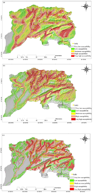
Assessment of erosion susceptibility using SVM and BRT models and their validation
To predict gully erosion, the maps of erosion susceptibility were generated based on the results of the SVM and BRT algorithms and the related conditioning factors. These maps exhibited five susceptibility degrees for gullying (Figure 5). The gully erosion susceptibility map obtained from the LN-SVM model illustrated that 24.51% of the watershed area experienced very high susceptibility, while 24.49% and 7.01% of the watershed area exhibited low and very low susceptibility, respectively (Figure 5a). The results of the RBF-SVM model exhibited that 9.94%, 41.14%, 7.15%, 7.46%, and 34.30% of the watershed have very low, low, moderate, high, and very high susceptibility, respectively (Figure 5b). Further, based on the results obtained from the BRT model, 9.64%, 24.33%, 34.84%, 7.44%, and 26.42% of the watershed have very low, low, moderate, high, and very high susceptibility, respectively (Figure 5c).
The results of the two machine learning algorithms successfully assessed the gully erosion-prone areas within the watershed (Figure 6). The validation results (AUC values) for discriminating the predictive performance of the models illustrated that the two machine learning models were very good for delimiting gully-prone areas with high accuracy. The BRF-SVM (AUC= 0.89) was the most robust model, illustrating the best prediction rate, while LN-SVM did not show an acceptable accuracy (AUC= 0.77). The BRT model (AUC= 0.85) was the second optimal model for predicting erosion susceptibility in the region. Furthermore, the AUC values of training datasets were 0.96 for the BRF-SVM model and 0.95 for the BRT model. Further, the results of statistical indices associated with the reliability of the models (RMSE and R2) illustrated that the model of BRF-SVM, followed by BRT had the lowest RMSE and the highest R2 (i.e. the most reliable models to assess the gully erosion-prone areas) compared with the LN-SVM (Table 4).
Table 4 Reliability of model accuracy based on the coefficient of determination (R2) and root mean square error (RMSE)
| Model | Train Data (70%) | Validation Data (30%) | ||
|---|---|---|---|---|
| R2 | RMSE | R2 | RMSE | |
| SVM (Linear Kernel) | 0.34 | 0.43 | 0.13 | 0.46 |
| SVM (Radial Basis Function) | 0.91 | 0.23 | 0.76 | 0.32 |
| BRT | 0.83 | 0.29 | 0.64 | 0.38 |
Nonparametric methods such as SVM and BRT are appropriate approaches to solve problems related to modeling. These algorithms can manage the collinear relationship among conditioning factors. Other researchers (Amiri et al., 2019) expressed that the most important advantage of the BRT is eliminating variables with a large number of missing values compared with other models. As some studies showed (Pourghasemi et al., 2017; Marjanovic et al., 2011), the improvement of the AUC values for validation and train data in different replicates is the most important advantage of the support vector machine algorithm. This characteristic caused this model could handle complex and nonlinear relationships, in comparison with models such as the artificial neural network. The findings of this study showed that the models of SVM and BRT with considering the interaction between independent variables could appropriately model gully erosion-prone areas with a high accuracy, as other studies reported (Gayen et al. 2019; Rahmati et al., 2017; Elith et al., 2008). Overall, the gully erosion susceptibility maps could provide an appropriate strategy for geo-conservation and restoration efforts in gully erosion-prone areas within the study watershed.
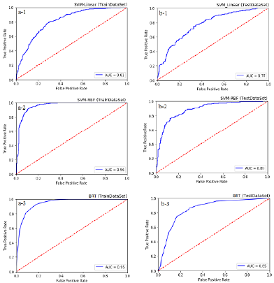
Figure 6 The area under the curve (AUC) based on train (a1-a3) and validation (b1-b3) datasets for discriminating the accuracy of LN-SVM, RBF-SVM, and BRT models
The interactions among various variables such as terrain indices, lithological characteristics, and land use/cover changes affect linear erosion development as rilling and gullying, which irreversibly threaten the health and resilience of soil systems. This study shows the results obtained by applying two machine learning methods for predicting the gully head cut susceptibility in northern Iran, as the second country in the world in terms of soil erosion. Mean annual soil losses caused by the gully erosion in this country estimate approximately 2.5 billion tons. These models can be appropriate tools to understand mechanisms controlling gully erosion and, therefore, can help to implement geo-conservation and management efforts for mitigating disasters associated with this hazard.
Conclusions
Soil degradation induced by gully erosion is the most critical challenge faced by many of the world's dryland regions. Although this hazard occurs on a small scale, its consequences will have a substantial impact on global scales, for example, the impacts of gully erosion on the degradation of a large amount of OC-rich topsoil that is combined with deeper horizons poor in OC. This event stimulates carbon mineralization and, subsequently, affects the exchange of carbon between the atmosphere and the pedosphere and associated instability in the carbon dioxide concentrations of the atmosphere. Therefore, to mitigate this hazard and the related environmental problems, it is necessary to understand the mechanisms controlling gully erosion. The results of this study showed the efficiency of two machine learning algorithms, including BRT and SVM, in the prediction of erosion susceptibility in northern Iran. Based on the results of the Boruta algorithm, slope gradient, land use, lithology, distance from river, elevation, river density, distance from fault, plan curvature, and SPI were the most effective factors that controlled the occurrence of gully erosion in the study region. Further, the results of the EBF model showed the spatial relationship among causative variables and gullied locations. Based on these findings, topographic thresholds for gully erosion tended to be lower on rangeland and weak textured soils, such as loess and marl. Furthermore, the spatial correlation of gullying with rangeland and weak textured soils within concave positions illustrated that the interactions among soil characteristics, topography, and land use could stimulate a low topographic threshold for gullying. The validation results related to the statistical indices of the reliability and discrimination accuracy of the models showed that the two machine learning models were very good for demarcating gully erosion areas with high accuracy. The BRF-SVM was the most robust model (AUC= 0.89; R2= 0.91; RMSE= 0.23), illustrating the best prediction rate. The BRT model (AUC= 0.85; R2= 0.83; RMSE= 0.29) was the second optimal model for predicting erosion susceptibility in the region. The gully erosion susceptibility maps could provide an appropriate strategy for geo-conservation and restoration efforts in gully erosion-prone areas within the study watershed.

