


 English (pdf)
 Article in xml format
 Article references
 Send this article by e-mail
 Cited by SciELO
  Cited by Google
  Similars in
SciELO
Similars in
SciELO  Similars in Google
 Permalink
1. Introduction
One of the important assignments of geodesy is the establishment of reference systems and constant improvements in their quality and accuracy, along with the advances in computational technologies and measurement instruments. This progress in spatial techniques enabled the positioning via a three-dimensional cartesian coordinate system associated with a conventionally defined ellipsoid. Consequently, the dynamic phenomena of the Earth caused by geophysical effects are quantified and qualified through two references, the Celestial Reference System and the Terrestrial Reference System, which are monitored by the International Earth Rotation and Reference Systems Service (see: https://www.iers.org/IERS/EN/Home/home node.html) (Blitzkow et al., 2011).
In the past two decades, low orbit satellite missions such as Challenging Minisatellite Payload (CHAMP) (GFZ, 2019), Gravity Recovery and Climate Experiment (GRACE) (JPL, 2011), and in particular the Gravity field and steady-state Ocean Circulation Explorer (GOCE) (ESA, 2009), addressed the attention to modeling the high frequencies of Earth the gravity field, reaching unprecedented results (for more details see: http://icgem.gfz-potsdam.de/home). Today, along with the improvement of Digital Terrain Models (DTMs) and terrestrial gravity measurements, the effort is toward establishing a height reference with physical meaning, the International Height Reference System (IHRS).
The physical and geometrical systems form the Global Geodetic Reference System (GGRS) whose importance is recognized and supported by the United Nations (UN). The United Nations General Assembly on a Global Geodetic Reference Frame (GGRF-UN) of Sustainable Development (A/RES/69/266) on February 26, 2015 reinforces the importance of a stable global geodetic reference structure to identify areas under threat from floods, earthquakes, or droughts, and to adopt preventive measures. The key to mitigating damage caused by natural phenomena, human activities, and carrying out sustainable planning is the implementation, among others, of a system of physical heights based on gravimetric data (United Nations General Assembly, 2015).
In addition to providing an infrastructure for the development of studies on a global level, the establishment of the IHRS is fundamental to correcting the deficiencies in the local height systems. The vertical networks around the world differ up to 2 m, making it difficult to interchange information between systems (Ihde et al., 2017). The correction of these inconsistencies is dependent on efforts to readjust the height network, perform gravimetric densification surveys, and evaluate the Global Geopotential Models (GGM) and Topographic Models in the study region. Since the framework of the IHRS is under discussion, it is pertinent to develop studies to identify the difficulties involving the methodology and information for determining the gravity potential values. The paper aimed to determine and compare the gravity potential values at four stations in Brazil, located in São Paulo state using two approaches. First, a numerical integration method with Hotine's kernel was performed using the radius of 110 km and 210 km around the station location. Second, the gravity potential was recovered from an existing and recent quasi-geoid model.
1.1 Study Area
The state of São Paulo is located in the southeast part of Brazil. Its size corresponds to 248.219,481 km2; its population is estimated at 46,289,333. The state has the bigger Gross Domestic Product (GNP) in the country (IBGE, 2019).
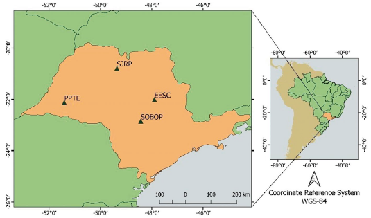
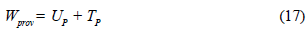
The proposed IHRF stations are located in the cities of Botucatu (SOBOP), Presidente Prudente (PPTE), São Carlos (EESC) and São José do Rio Preto (SJRP) (Figure 1). PPTE was already planned, by the Instituto Brasileiro de Geografia e Estatística (IBGE) for the global network, and the others are being suggested for regional infrastructure. They are placed in the same coordinates of Rede Brasileira de Monitoramento Contínuo dos Sistemas GNSS (RBMC), and close to them there are absolute gravity observations. The latter stations contribute to the International Gravity Reference System (IGRS), which is well underway, proposed by The International Association of Geodesy (IAG) in resolution No. 2 of 2015 (Drewes et al., 2016; Ihde et al., 2017; Tóth, 2017). The IGRS aims to replace the world gravimetric reference still used, the International Gravity Standardization Net 1971 (IGSN-71) network, whose precision and spatial distribution no longer satisfy the requirements to implement a global altimetric reference. The first studies suggest the optimistic precision of 1 a 2 µGal on the gravity measurements (Wilmes et al., 2015).
The state is quite complete in terms of 5' grid of gravity anomalies. Currently, it has about 9,257 gravimetric points. The first surveys were carried out in the 1970s by institutions such as the Instituto de Astronomia, Geofísica e Ciências Atmosféricas of Universidade de São Paulo (IAG-USP), Observatório Nacional (ON), Petrobrás, and the Anglo-Brazilian Gravity Project, carried out in conjunction with the University of Leeds and the IBGE (Castro Junior et al., 2018). Years after, thematic project number 06/04008-2, of the Fundação de Amparo a Pesquisa do Estado de São Paulo (FAPESP) gravimetric densification surveys for the production of an advanced geoid model were carried out (Guimarães et al., 2014).
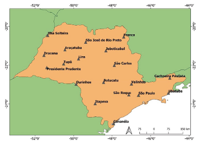
In 2016, a Gravimetric Reference System, compound of absolute measurements, was implemented in the state of São Paulo, from an initiative of the Laboratório de Topografia e Geodésia of the Escola Politécnica da Universidade de São Paulo (LTG/EPUSP), Instituto Geográfico e Cartográfico de São Paulo (IGC-SP), IBGE and Centro de Estudos de Geodesia (CENEGEO). This reference contains 15 new stations and four reoccupations (Cananéia, São Paulo, Ubatuba and Valinhos stations), distributed according to Figure 2. The measurements were performed using an absolute gravimeter Micro-g LaCoste, A-10, number 32, belonging to the IGC-SP and operating at the LTG. Gravity data information for download is available in Portuguese (see: https://www.cenegeo.com.br/rede-grav-absoluta/rede-absoluta-sao-paulo) and in English (see: http://bgi.obs-mip.fr/gravity-databases/).
2. International Height Reference System
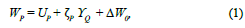
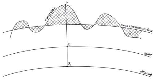
The IAG, motivated by the Global Geodetic Observing System (GGOS), proposed in resolution No. 1 of 2015 the creation of the so-called International Height Reference System with conventions for its definition (see IAG Resolution No. 1 (2015) in Drewes et al., 2016; Ihde et al., 2017; Tóth, 2017). The computation will be based on the mean value of the Earth's gravity potential, conventional adopted, W' = 62,636,853.4 m2s-2, (Sánchez et al 2016), and specific parameters to standardize the framework. In addition, this system, strictly based on the gravity field, will be related to International Terrestrial Reference Frame (ITRF) coordinates with its variation in time. The parameters, observations, and data must be related to the mean tidal system or mean crust, and the unit of length is the meter and the unit of time is the second in the International System of Units. The vertical coordinates are differences AWp, determined between the gravity potential at a given point P (W p ) and W 0 ; such differences in gravity potential are also referred to as geopotential numbers (Cp). The spatial reference of P position for the potential W = W(X) is related to the X coordinates of the ITRS (Figure 3). After the implantation of global references, the unification process will integrate the ocean topography, determined by the satellite altimetry technique, also considering the tide records.
The fundamental component of the IHRF is the GGM, described as coefficients of the gravitational potential function complemented with terrestrial gravimetric data. However, terrestrial gravimetric information is necessary and must be properly arranged around IHRF stations. For this, Sánchez et al. (2016) recommend that:
the gravity observations must be distributed around the IHRF reference station within a radius of 210 km;
the minimum accuracy of these values must be ± 20 uGal;
the gravity position point must be collected via Global Navigation Satellite Systems (GNSS) positioning;
in mountainous areas, there should be approximately 50% more gravimetric observations;
GGMs and DTMs uncertainties must be considered in the framework.
Three methods are proposed for computation (Sánchez et al., 2021): based on geopotential models of high-resolution, containing gravity and topographic information; using precise regional geoid or quasi-geoid based on the gravity field, and vertical datum unification using the local height systems based on the solution of Geodetic Boundary Value Problem (GBVP).
The first approach is a direct way that consists in determining W p by inserting ITRF coordinates in a reliable harmonic expansion tool such ICGEM (Ince et al., 2019) or any other GGMs software. There is a limitation of this methodology due to the poor accuracy of GGMs in some areas. Well-surveyed areas expect a Root Mean Square (RMS) difference of ±4 cm (Rummel et al. 2014), comparing the Global Positioning System (GPS) determinations on the leveling network and GGMs models elements. While others with sparse gravity data can reach 1 m (Drinkwater et al., 2003; Sánchez and Sideris, 2017). This occurs because in regions with scarce gravimetric information, the GGMs use brings up the so-called omission error, responsible for affecting its accuracy above 300 degrees (Rummel et al., 2014).
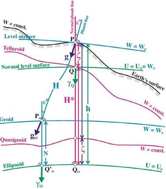
Figure 3 Gravity field quantities represented within a height reference. Source: (Sánchez et al., 2021).
The second method consists of determining the gravity potential using geoid or quasi-geoid models. The precise regional gravity field model provides geoid undulation (N p ), case of a geoid, or height anomaly ( Z p ) referred to the quasi-geoid (used in this paper). Thus, W p value (Figure 3) can be determined (Sánchez et al., 2021):
rewriting:
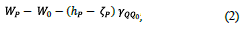
where, U p is the normal potential at point P;Yq the normal gravity acceleration at point Q; h p is geodetic height; ү QQ0 is the normal gravity at the telluroid between Q and Q 0 points. Using the geoid model (N p ) (Sánchez et al., 2021), (2) becomes:
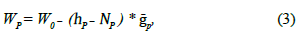
with mean gravity acceleration gp (Hofmann-Wellenhof & Moritz, 2006):

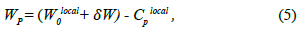
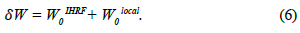
using the real gravity acceleration g p and the terrain correction TC p The vertical datum unification methodology aims to determine the difference between W 0 and the local W 0 local to correct the regional geopotential numbers (C 0 local ). Thus, is given by:
with the potential gravity difference given by difference δW:
In this latter approach, different strategies can be used to determine a W p value. Usually, the fixed GBVP or the scalar-free GBVP are solved using numerical integration. Recently, least-squares collocation and spherical radial basis functions are also used (Sánchez et al., 2021).
3. The modeling of topographic surfaces for the RTM
The computation of anomalous field elements with centimeter accuracy requires the decomposition of them into different wavelengths: long, medium, and short. The RTM technique consists of using a high-resolution DTM to compute the topographic effects to apply them in the spectral decomposition. The wavelengths are segmented with the remove-restore technique, also considering the contribution of the low frequencies of the gravitational signal, determined by a geopotential model. In the methodology described in Forsberg (1984), the topographic effects are quantified using a digital terrain model of the average elevations of the terrain, called the reference DTM (Forsberg & Tscherning, 2008), produced according to two DTMs, one of high and one of low resolution. The latter is also named irregular DTM. The model, called the reference DTM, is defined by a low-pass filter, produced according to the moving average operator corresponding to the distance over which the heights will be averaged.
The DTM needs to have a resolution compatible with the spherical harmonic function coefficients of the gravitational potential from the GGM (Forsberg & Tscherning, 2008). In other words, the order and degree of the GGM must correspond to the spatial resolution of the DTM, thus the topography is properly quantified by the long and short wavelengths.
The topographic effects (ΔARTM) is determined using the expression (7), considering as approximation a rectangular prism with mass density (p) of the surface rocks of the continental crust (2.67 gem-3) and surface (1.03 gem-3) (Tziavos & Sideris, 2013).
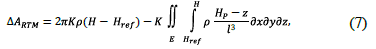
where, H ,is the height of the reference DTM used, H is the height of the topographic masses defined by the high-resolution DTM, H p is the normal height of the point, К is the gravitational constant, / corresponds to the integration distance, and ∂X∂Y∂Z is the element of differentiation for the volume.
The DTM SRTM15+ with a resolution of 15 arcsec, was the model chosen for the application of the RTM technique due to its availability for the area of the continent and the ocean. The SRTM15+ is derived from the Shuttle Radar Topography Mission and supplemented with data from the Advanced Spaceborne Thermal Emission and Reflection Radiometer, known as ASTER mission (Fair et al., 2007). In the ocean, this model has data derived from the CryoSat-2 and Jason-1 missions (Tozer et al., 2019).
As mentioned, computing the RTM requires three DTMs. The irregular model, formatted in a 3' grid, was determined in the SELECT program, developed by Forsberg & Tscherning, (2008) from the high-resolution DTM, the SRTM15+. The reference model was produced in the TCGRID program, based on the two previous models. The latter is a grid with the mean height, generated from a low-pass filter filtered with the moving average operator.
The production of the reference DTM is dependent on the spatial resolution of the GGM whose computation depends on the choice of the degree and the order of the coefficients developed in a series of spherical harmonic functions of the gravitational potential. To compute the gravity potential, the GOCO05S GGM was chosen with nmax: 100 and 200 due to its composition and the well fit on the GPS/leveling benchmarks of Brazil (Fecher et al., 2017; Nicacio & Dalazoana, 2018). The degree and order of the GGM can be expressed according to the expression (8), (Torge & Müller, 2012):
Based on the order and degree of the chosen GGMs, tests were performed in the TCGRID and TC programs Forsberg & Tscherning (2008). The TCGRID routine computes the reference surface according to the irregular DTM (3') and by choosing odd values for the moving window. In the first instance, sixteen reference surfaces were computed using odd values from 1 to 31. These values determine the window's search radius for applying the low-pass filter (Table 1 ). To optimize, the DTMREF-RTM program developed at EPUSP was used to determine the best resolution for each type of residual, based on the lower RMS difference residuals (Figure 5 and Table 2).
Table 1 Spatial resolution of the moving window.
| Factor | Minutes | Degree | kin |
|---|---|---|---|
| 1 | 3 | 0.05 | 5.6 |
| 3 | 9 | 0.15 | 16.7 |
| 5 | 15 | 0.25 | 27.8 |
| 7 | 21 | 0.35 | 38.9 |
| 9 | 27 | 0.45 | 50.0 |
| 11 | 33 | 0.55 | 61.1 |
| 13 | 39 | 0.65 | 72.2 |
| 15 | 45 | 0.75 | 83.3 |
| 17 | 51 | 0.85 | 94.5 |
| 19 | 57 | 0.95 | 105.6 |
| 21 | 63 | 1.05 | 116.7 |
| 23 | 69 | 1.15 | 127.8 |
| 25 | 75 | 1.25 | 138.9 |
| 27 | 81 | 1.35 | 150.0 |
| 29 | 87 | 1.45 | 161.1 |
| 31 | 93 | 1.55 | 172.3 |
Table 2 Chosen moving window for reference DTM.
| GGM | nmax | Factor | RMS |
|---|---|---|---|
| GOCO05S | 100 | 21 | 11.84 |
| GOCO05S | 200 | 13 | 8.74 |
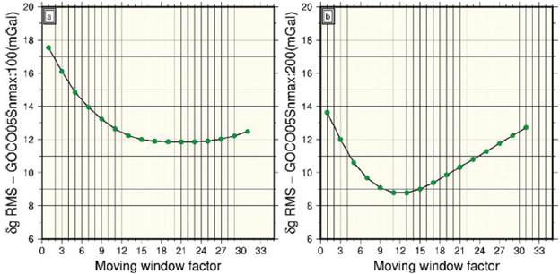
Figure 5 RMS of residual gravity disturbance for each factor (a: GOCO05S nmax: 100; b: GOCO05S nmax: 200.
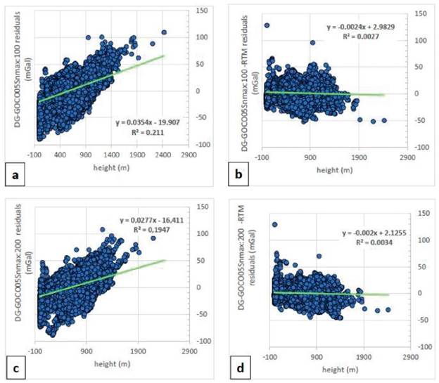
Figure 6 shows the residual gravity disturbance before and after applying the RTM for grid 100 (a and b) and 200 (c and d), respectively. The RTM represents a gravity disturbance with respect to topography, when removing it, the residual gravity disturbance becomes independent of terrain effects. This is observed by the determination coefficient shown in this figure. The nmax: 100 solution has a residuals variance of 21% dependent on the height. Reducing the topographic effects, R 2 results in 0.2%. Whereas for nmax: 200 the residuals have a variance of 19% in relation to the height, and considering the RTM, it decreased by 0.3%.
4. Determination of the gravity potential
4.1 Gravity potential values by GBVP solution
The gravity potential was computed by solving the fixed GBVP. In this task gravity disturbances (9) were determined by gravity acceleration and coordinates (φ, λ and h) point data. They were transformed to zero-tide system according to Sanchez & Sideris (2017).

In Neumann's GBVP, the Hotine kernel, also called Neumann Koch's formula, is used. The disturbing potential is defined according to the expression (10) (Hofmann-Wellenhof & Moritz, 2006):
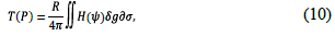
with the Hotine-Kochi7 (\\r) kernel expressed by:
То compute (9), it is necessary a normal gravity acceleration value at a point on the physical surface. For this, the ANOMALIA MOLODENSKY routine, developed at EPUSP, was used. This program performs the computation using the strict upward continuation described in Heiskanen & Moritiz (1967), with the parameters of the Global Reference System 1980 (GRS80) ellipsoid. Gravity disturbances were also corrected for atmospheric effects described in Wenzel (1985).
In general, computing the gravity potential at a point, through numerical integration, requires data distribution in an area of 210 km. This extension offers limitations for smaller countries, regions with difficult access, and coastal areas, such as the Brazilian IHRF stations: Fortaleza and Imbituba.
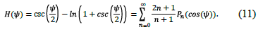
Figure 7 Residual gravity disturbance (mGal) (α-using the GOCO05S nmax:100; è-using the GOCO05S nmax:200).
An adequate radius to determine a W p value should integrate an appropriate methodology to ensure the spectral transfer of the residual gravity field, as well to quantify and to remove the terrain effecs. (Torge & Muller, 2012). The harmonic coefficients of GGMs, expressed in degree and order, represent the spectral resolution and can also be converted into a spatial resolution.
In agreement with the expression (8), regions with gravimetric data in a radius of 210 km used a GGM up to nmax: 100. While areas of 110 km used GGM up to nmax: 200.
Besides, Ihde et al. (2017) suggest for the IHRF framework, as well as the applications that involve high precision, it is sufficient to choose a model that contains only satellite data and that has a homogeneous approximation of the long wavelength of the Earth's gravity potential.
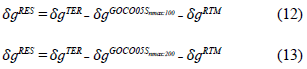
According to the suggestion above, expressions 12 and 13 show how the residual gravity disturbance have been defined, for degree 100 and 200, respectively. The second term of the right side corresponds GOCO05S long wavelengths. The last term is partial short wavelengths obtained by RTM with the selected DTM (see Section 3).
The results of the remove step on the gravity disturbances are shown in Figure 7. As can be seen, GGMs contribute differently depending on the degree and order. In this case, the systematic component is smaller for nmax:200, compared to the use of the MGG with nmax: 100, as expected. This behavior is observed at Table 3 in the residual mean.
5. International Height Reference System
Both data were interpolated using the moving average operator in a 5'x5'grid with the SELECT software. The short wavelength components of the disturbing potential T res were determined using the HOTINE 5MIN software, developed at EPUSP. It computes the short wavelengths of T res according to the chosen area, using the modified Hotine-Koch integral. The input data are the residual gravity disturbances and the output file provides a residual disturbing potential value.
The restore step was performed with the HARMEXP program, which belongs to the GRAVSOFT package (Forsberg & Tscherning, 2008). Analogously to the remove step, the model used was GOCO05S with the degree and order 100 and 200, according to the integration radius 210 or 110 km, respectively. The software computes the normal gravity acceleration for each station and ζ GGM , Applying the expression 14, the T GGM was obtained.
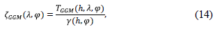
where T GGM is the disturbing potential of the GGM and y is the normal gravity acceleration at the given point (h,λ, φ).
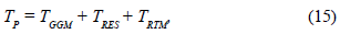
Short wavelengths, referring to the RTM, were determined with the TC program for each station. In this step, the RTM was computed with the residual height anomaly using the same DTMs as in the remove step and transformed in order to apply in the T RES . The final disturbing potential was expressed by:
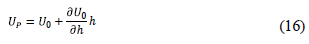
The normal gravity potential was defined using the POTENCIAL_ NORMAL program developed by EPUSP. The routine determines U p , expression (16), from the normal gravity acceleration, the geodetic height, and the GRS80 parameters.
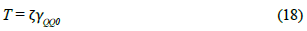
The provisory gravity potential (W prov ), given by the sum of disturbing
potential and the normal potential, was expressed by (17):
Section 5.2.1 shows the results: potential in zero-tide (W ZT ) and geopotential number consistent with the mean-tide (C IHRF ).
5.1 Disturbing potential differences of the numerical integration approach using H otine 's-Koch kernel
The disturbing potential for the stations obtained in three steps (5) by Hotine's methodologies is shown in Table 4. It was added -1.73 m2s-2, obtained by (15), for the zero-degree term in the in the T p final values (see Section 5.2.1 and Table 6).
The T p final values computed in the different remove-restore methodologies have a high dependence on long wavelengths. In addition, Т GGM values show significant differences between order and degree 100 and 200. Silva (2021) studied the RMS difference between height anomalies, obtained from the GPS determinations on the leveling network, and the GOCO06S geoidal height of 86 points located in São Paulo state. In the study was observed a difference of 20 cm approximately, between degrees 100 and 200. On the other hand, the homogeneous distribution of gravimetric data and the use of RTM tend to reduce this difference between solutions.
The state of São Paulo is characterized by topographical heterogeneities (Fig.8) which can influence the GGM. The SPBO station region has irregular topography of approximately 1,000 m. Whereas, PPTE is located in an area of homogeneous topography, compared to the SPBO station, with elevations of approximately 900 m in the southern region. EESC station presents irregular topography of up to 1,500 m and the topography around the SJRP is smoother compared to other stations.
Table 4 Residual disturbing potential (m2s 2).
| Solution | Hotine nmax: 100 | Hotine nmax:200 | ||||||
|---|---|---|---|---|---|---|---|---|
| Stations | T res | T ggm | Trtm | T p final | T res | T ggm | Trtm | T p fina |
| SBPO | 1.526 | -50.156 | 0.028 | -50.328 | -1.188 | -48.654 | 0.017 | -51.551 |
| EESC | -0.437 | -55.908 | 0.039 | -58.031 | 0.280 | -60.885 | 0.038 | -62.292 |
| PPTE | -1.636 | -50.397 | -0.021 | -53.780 | -0.465 | -46.576 | -0.002 | -48.769 |
| SJRP | -0.416 | -64.854 | -0.028 | -67.023 | 0.123 | -65.393 | -0.006 | -67.001 |
For the SPBO station, the Т GGM values differ by -1.502 m2s-2 between nmax: 100 and 200 and for T p final values, 1.223 m2s-2. In short, there is a contribution of the gravimetric and topographic components to reduce discrepancies between solutions.
Comparing the T p final results of EESC, a difference of 4.261 m2s-2 corresponding to 43 cm, is observed between degree and order 100 and 200. These discrepancies are related to the long-wavelength component because it has a similar difference of4.977 m2s-2, or 51 cm.
The results of T p final for PPTE show that the difference between degree and order is -5.011 m2s-2. The values of Т MGG used in the restore step (Table 4), differ by 3.821 m2s-2 between degree and order 100 and 200. The results showed an inverse behavior increasing the discrepancies of different order and degree, suggesting a trend in the terrestrial gravity data or on the DTM. On the other hand, studies carried out by Ribeiro et al. (2021) for the PPTE, used the GOCO05C model developed up to nmax: 250, without application of the RTM, showed 0.470 m2s-2 or 5 cm of difference, considering the performance of the IHRF with degree and order 200.
In SJRP, the results of the disturbing potential showed a discrepancy of -0.022 m2s-2, corresponding to 0.2 cm, between solutions of different degrees and order. Unlike the other stations, the convergence of the results in SJRP was possible due to the small difference between the long-wavelength components of the GOCO05S, corresponding to 5 cm.
5.2 Recovering potential gravity values from existing quasi-geoid model
The multiple ways to solve the GBVP and the complexities involving kernel s and gravity data availability lead to implementing the IHRF computation, using gravity field modeling through the determination and/or modification of geoid models. Recently, computation strategies have been studied to separate and quantify the contributions of elements in terms of method and input data (Sánchez et al., 2021). After that, the approach will be standardized to get a uniform solution using distinct methods.
In this paper, a quasi-geoid model of São Paulo (Silva et al., 2021), which has the same database used in Hotine's methodologies, was used. The was computed using the GRAVSOFT package (Forsberg & Tscherning, 2008). The approach was the numerical integration through the Fast Fourier Transform (FFT) using Molodensky gravity anomaly in a 5'x5' grid. The RCR was applied using RTM technique and the XGM2019e global gravity model truncated at degree and order 250. Its validation showed an RMS difference of 18 cm with 298 benchmarks with GPS and normal height.
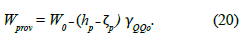
The first step in recovering the height anomaly of the quasi-geoid was interpolating ζ in the IHRF proposed station, in which the geodetic coordinates are from an RBMC. Through the relation 18, we had the disturbing potential:
where, Yqq 0 is given by:

φ,h ζ Çare respecting the geodetic latitude, geodetic height, and the height anomaly of the computing point. The constants parameters are the flattening (/), major semi-axis (α), physical constant and the gravity acceleration in the ellipsoid (m), for the GRS80 according (Moritz, 2000).
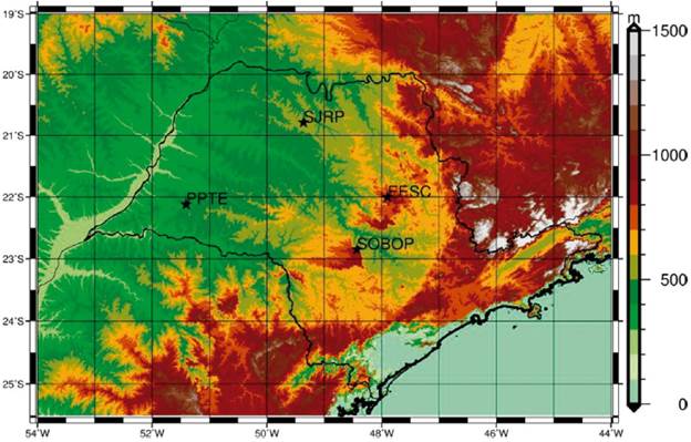
Using W 0 = 62,636,853.4 m2s-2, the W pro was obtained by (Sánchez et al, 2021):
The used elements, in the zero-tide system, are shown in Table 5.
Table 5 Elements used in the quasi-geoid's solution.
| Stations | ζp(m) | Ү QQO (mGal) | h p (m) |
|---|---|---|---|
| SBPO | -5.287 | 9.7868921880 | 803.138 |
| EESC | -6.136 | 9.7863172519 | 824.614 |
| PPTE | -4.853 | 9.7869990406 | 431.075 |
| SJRP | -6.992 | 9.7860126043 | 535.933 |
5.2.1 Permanent tide and zero-degree term
IAG Resolution No. 1 (2015) introduces the mean-tide system to support the geodetic monitoring of geophysical phenomena governed by fluids within the System Earth. For instance, the sea level change monitoring is performed in the mean-tide system, because removing the direct or indirect effects of the permanent tide misrepresents the real water motion and does not allow a reliable quantification and modeling of the sea-level change. This occurs not only in océanographie applications but also in hydrographie and geophysical fluid studies. In other words, the global change occurs in the mean-tide system and the IHRF should provide a consistent reference in monitoring it. However, considering that gravity field modeling is not possible in the mean-tide system (because the gravity potential would not be a harmonic function), it is agreed that the data processing is performed in the tide-free or zero-tide system, and then, at the very end of the process, the IHRF coordinates are converted to the mean-tide system (Sánchez et al, 2021). In this paper, the coordinates and GGM are tide-free and zero-tide systems, respectively. Therefore, the scheme for the determination of IHRF geopotential was computed following Mäkinen (2021).
The final gravity potential is obtained by:
Since the coordinates system was given in tide-free ITRF2021, the correction ΔW ITRF must be added to obtain the potential at the mean-tide = zero-tide position:

The geopotential number consistent with the mean-tide is obtained by:
Where geopotential number in zero-tide system (CZT) is computed by:

and gravity potential in mean-tide is:

The gravity field components should be given in the Geodetic Reference System of 1980 (GRS80). Since the geocentric gravitational constant (GM) of the latest GGMs differs from the GRS80, it is necessary to apply the correction, called zero-degree term. Thus, the GM difference is adjusted, as well as the discrepancy between the gravity potential W' and the normal gravity potential U 0 as follow:
where, r p is the geocentric radial distance of the computation point, ΔW 0 is the difference between the normal potential (U 0 ) at ellipsoid for GRS80 and conventional value W g equal 62,636,853.4 m2s-2.
The values for permanent tide corrections and the zero-degree term are shown in Table 6. The ζ 0 T (m2s-2 units) is the zero-degree term, it was added to obtain the T p final , case of Hotine's solutions (see Section 5.1 and Table 4). It is computed by expression 23 without ү Q
5.2.2 Gravity potential (W ) and geopotential number (C IHSr ) for São Paulo stations
Table 7 shows the gravity potential and geopotential number obtained numerical integration method with Hotine's kernel (nmax=100 and 200) and quasi-geoid (nmax=250). Figures 9 and 10 show and the differences between geopotential numbers for the three solutions, respectively.
Table 7 Gravity potential and geopotential number for Hotine's solution (m2s-2).
| Solution | Hotine nmax: 100 | Hotine nmax:200 | Quasi-geoid nmax:250 | |||
|---|---|---|---|---|---|---|
| Station | W ZT 100 | C IHRF 100 | W ZT 200 | C IHRF 200 | W ZT QG | C QG IHRF |
| SBPO | 62,628,949.67 | 7,902.871 | 62,628,948.44 | 7,905.168 | 62,628,941.10 | 7,911.437 |
| EESC | 62,628,732.27 | 8,120.220 | 62,628,728.01 | 8,125.615 | 62,628,723.07 | 8,129.420 |
| PPTE | 62,632,587.65 | 4,264.842 | 62,632,592.66 | 4,260.957 | 62,632,586.63 | 4,265.866 |
| SJRP | 62,631,548.67 | 5,303.755 | 62,631,548.69 | 5,304.950 | 62,631,539.96 | 5,312.462 |
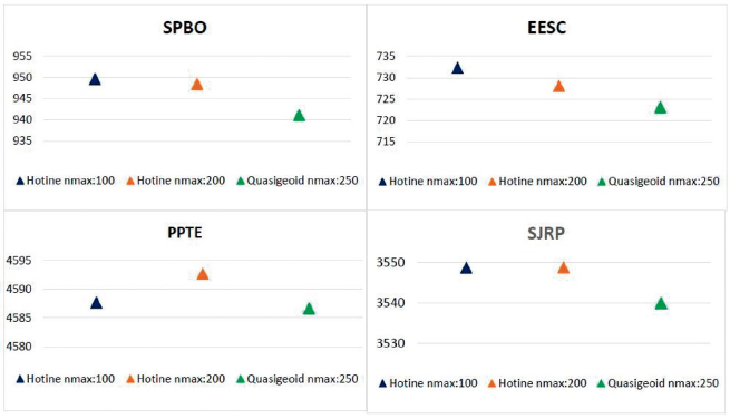
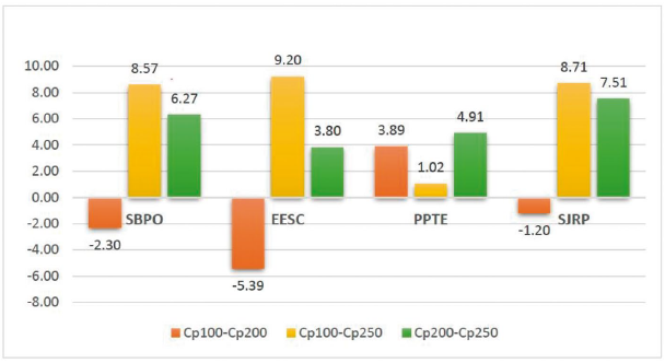
Comparing C 100 IHRF and C 200 IHRF with C QG IHRF , the stations SPBO and SJRP show discrepancies around -8.57 m2s-2 and -7.34 (-87 and -75 cm approximately), respectively. However, these discrepancies in EESC are -9.20 m2s-2 (94 cm) and -4.94 m2s-2 (-50 cm). For PPTE, these are -1.02 m2s-2 (10 cm) and 6.03 m2s-2 (62 cm).
It is worthy to mention all the final solutions have the order degree term as well they are in the same tide system, mean-tide according to Mäkinen (2021) and Sánchez et al. (2021)). The values obtained suggest heterogeneities of the used approaches. The quasi-geoid model suffers the influence of 2 degrees beyond the area of São Paulo. On the other hand, in Hotine's methodology, the integration area is smaller and with gravity coverage complete in a 5'grid. In addition, for the quasi-geoid model nmax:250 (Silva et al., 2021) the voids were filled with XGM2019 nmax:2190.
Final Remarks
The efforts performed in the last years to define the IHRF and to include it on the Global Geodetic Reference Frame for Sustainable Development, recognized by the UN, already brought important advances. Countries start to update their height system to implement the IHRF and to improve their infrastructure. Nevertheless, challenges remain concerning the computation methodology. This paper aimed to contribute to IHRF studies by computing the gravity potential and geopotential number in stations with adequate gravimetric measurements to evaluate the numerical integration method with Hotine's kernel and an existing quasi-geoid model.
In the Brazilian case, the values found for in the different remove-restore methodologies have a dependence on long wavelengths. The gravitational components of the GGMs showed significant discrepancies with distinct order e degree and in divergent ways for each station. Considering the RMS difference (20 cm) between nmax:100 and 200 with the leveling benchmarks in the state with the GOCO06S, the stations of EESC and PPTE has W p differences up to 20 cm.
The convergence between solutions with different degree and order only occurred for the SJRP station, where the difference between degree and order was 5 cm. Thus, it suggests that it is acceptable to compute IHRF in an area consisting of homogeneous gravimetric data in a radius of110 km, provided that the GGM is well representative for the area. On the other hand, PPTE station presented the smallest difference (5 cm) between the quasi-geoid methodology and Hotine approach with nmax: 100.
The state of São Paulo is one of the best regions with gravimetric coverage in South America. However, the current gravimetric coverage, DTMs, and GGMs are far to achieve the optimistic precision of 1 cm required for the IHRF.
There will be a long way to go towards establishing a terrestrial gravimetric infrastructure and including this data in digital models. On the other hand, the justification for the variations in the magnitudes of the anomalous field in the GGM long-wavelength requires a detailed analysis of multiple factors such as the geomorphological formation and the hydrological characteristics of the region. In addition, further studies should be performed using high-resolution DTM's and using different GGMs models.

