


 Inglés (pdf)
 Articulo en XML
 Referencias del artículo
 Enviar articulo por email
 Citado por SciELO
  Citado por Google
  Similares en
SciELO
Similares en
SciELO  Similares en Google
 Permalink
1. Introduction
The reciprocal bearing angles are exactly 180 degrees different on the plane. Unlike the plane on the sphere surface, the difference between reciprocal bearing or azimuth angle is approximately 180 degrees. Therefore, while a single bearing angle is sufficient in plane calculations, it is desired to find reciprocal bearing or azimuth angles separately on surfaces such as spheres and ellipsoids. Classic the bearing calculation or the azimuth calculation formulas only work correctly if the side is in the 1st quarter. If the side is located in the other quarters, the angles of the bearing or azimuth should be examined. For example, if the angle value given by the arctan function is positive, the bearing or azimuth angle is in the 1st or 3rd quarter. If the angle value is negative, the angle is in quarter 2 or 4. In order to find the value of the angle as univocal, the angle values found from the classical formulas need to be examined. Bearing or azimuth angles are critical in geodetic calculations. It is impossible to produce correct position information with wrong bearing or azimuth angles. Calculation of angles is done with the inverse (second) geodetic problem. While solving the inverse geodetic problem in order to find reciprocal bearing or azimuth angles, first, the angle from 1 to 2 is found. As a result of the analysis, if the 1st bearing or azimuth angle is wrong, it is likely to be wrong in the opposite (from 2 to 1) bearing or azimuth. In the proposed method, reciprocal bearing or azimuth angles are obtained independently and directly.
In our literature research, we came found some studies only for determining plane bearing angle (Antes, 1990; Breuer et al., 1985; Gellert et al., 1972) demonstrated direct bearing angle determination in the plane without quarter analysis. Hekimoğluglu (1991) also examined the condition problem and the direct formulas. We could not find any studies that give a direct bearing and azimuth angle on the spherical surface.
Formulas that give a direct azimuth angle on the sphere surface without examining the quarter with geographical coordinates are shown by the author in (Bektas, 2019; Bektas, 2021).
For the first time, in this study, formulas that give a direct bearing angle without examining the quarter with Soldner coordinates on the sphere surface will be discussed.
On the other hand, a solution proposal will be given against the division by zero errors in the bearing and azimuth angles calculations.
In this paper, firstly, bearing and azimuth angle, meridian system and Soldner coordinates on sphere will be mentioned in order to form a basis for the subject. After the relationship between azimuth, bearing angle and meridian convergence is given, direct azimuth angle determination with geographical coordinates, then direct bearing angle determination with Soldner coordinates will be discussed.
2. Direct Azimuth Angles with Geographical Coordinates
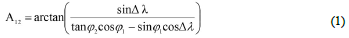
Classically, the reciprocal azimuth angles (A12, A21) from two points whose geographic coordinates P1(φ1, λ1), P2(φ2,λ2) are given obtained from the following formulas (Fig.1).
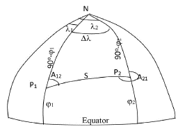
It is important to remember that these classic formulas only work correctly if the side is in the 1st quarter. If the side is located in the other quarters, the angles of the bearing angle should be examined. The necessary additions should be made for correct angles according to Table-1 seen below.
Table 1 Fixed value to add for azimuth angles
| Quadrant | Δφ=φ2−φ1 | Δλ=λ2− λ1 fixed | fixed value to add A12 | fixed value to add for A12 |
|---|---|---|---|---|
| 1.Quadrant | + | + | - | - |
| 2.Quadrant | + | - | + 180° | + 180o |
| 3.Quadrant | - | - | + 180° | -180o |
| 4.Quadrant | - | + | +360o | - |
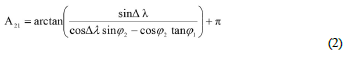
In this proposed method, formulas are given for obtaining the azimuth angle directly without any examination. For direct determination of azimuth by geographic coordinates, we provide the below formulas. In this proposed method, formulas are given to obtain the azimuth angle directly without any examination. The proposed method can calculate direct azimuth angles on the sphere and ellipsoid surface (Bektas, 2019).
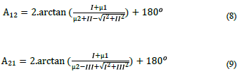
The given formulas in Equations 6 and 7 do not work if the denominator equals zero. The program will be interrupted because division by zero is done. This problem also arises in the use of classical formulas. In order not to interrupt the program, very small numbers are added to the numerator and denominator at a rate that will not affect the result. If µ1=1E - 15,... µ2 =1E - 27,... are selected, ten digit sensitive bearing angle values are obtained (Hekimoğlu, 1991). The division by zero error will be avoided if the following formulas (Eq. 8 and Eq. 9) are used.
3. Direct Bearing Angles with Soldner Coordinates in Meridian System on Sphere
This meridian system, as the name suggests, is based on the meridian. The meridian that defines the system is called the prime meridian, and a meridian near the study area is taken as the prime meridian (Heck, 2003).oSoldner coordinates system, have found wide application in geodesy. In particular, the Soldner coordinates system constitutes a suitable base for projection of the ellipsoid and the sphere. Soldner coordinates can be used in Cassini-Soldner projection without any processing.
In this system, the x-axis is the selected prime meridian (Figure 2). The coordinates of a point P1 on the sphere in the meridian system are defined as follows. The spherical distance (arcs of a great circle) from the P1 point to the prime meridian (P1F1) is the y value of the P1 point (y1 = P1F1).
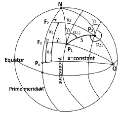
The distance of the perpendicular point F1 to the starting point Po on the prime meridian also gives the x coordinate (x1 = PoF1). The starting point of Po can also be taken on the equator.
These sides used in the calculations on the sphere s, y1, x1, y2, x2 in Figure 2 must be arcs of a great circle. Point O in Figure 2 becomes the pole of the prime meridian circle. So it is always OF1= OF2 = OPo = ϖ/2. In the Soldner coordinate system, the reference direction of the bearing angles of the sides is the parallel y=constant circle drawn to the prime meridian at that point (Figure-2). The prime meridian determines the Soldner system. Each meridian system creates a separate coordinate system. The ordinates of the points (y) to the left of the prime meridian are negative. Likewise, the abscissas of points (x) below the starting point take negative values. The azimuth angle is used for the direction values of the sides in main problem solutions with geographical coordinates. The azimuth angle (A12, A21) is the angle from the north wing of the meridian at a point to the clockwise side (Fig. 2).
The bearing angle is used for the direction values of the sides in main problem solutions with Soldner coordinates meridian system. The bearing angle (α12, α21) is from the north wing of the parallel to the prime meridian at a point to the clockwise side (Fig. 2).
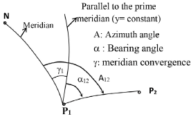
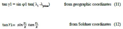
There is a meridian convergence ( γ ) between bearing and azimuth angle (Fig. 3). Meridian convergence can be easily calculated from the geographic or Soldner coordinates of the point. If the bearing angle (α) is given, it is converted to the azimuth angle by using the meridian convergence at that point

For example, γ 1 meridian convergence on the P1 point
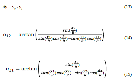
Reciprocal angles between two points whose coordinates are given in geodesy are obtained by solving the inverse (second) geodetic problem. Classically, the reciprocal bearing angles (α12, α21) from two points whose Soldner coordinates P1(y1, x1), P2(y2, x2) are given obtained from the following formulas (Fig. 4). Solving P1P2O spherical triangle
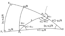
The bearing angle values found from the classical formula need to be examined. According to the quarter where the angle is located, the additions in the Table 2 below should be made.
Table 2 Fixed value to add for bearing angles
| Quadrant | Δу=У2- y1 | fixed value to add for α12 | fixed value to add for α21 |
|---|---|---|---|
| 1 and 2 | + | 90o | 270o |
| 3 and 4 | - | 270o | +90o |
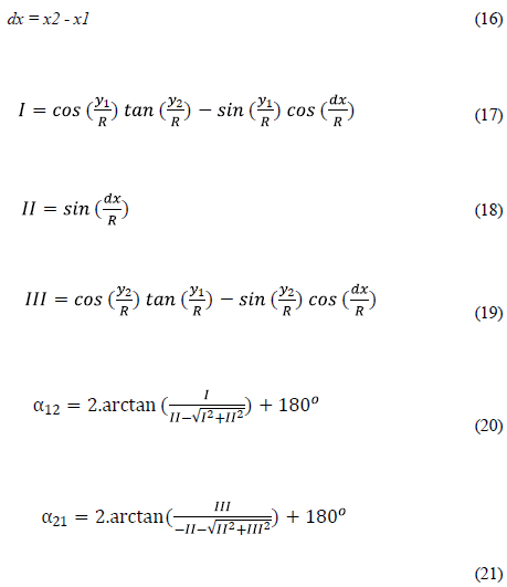
The following values of I, II and III are calculated to find the direct bearing angle without examining the sphere surface.
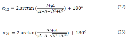
The given formulas in Equation 20 and Equation 21 do not work if the denominator equals zero. The program will be interrupted because division by zero is done. This problem also arises in the use of classical formulas. In order not to interrupt the program, very small numbers are added to the numerator and denominator at a rate that will not affect the result. If µ\1=1E - 15,... µ2 =1E - 27 are selected, ten-digit sensitive bearing angle values are obtained. The division by zero error will be avoided if the following formulas Equation 22 and Equation 23 are used.
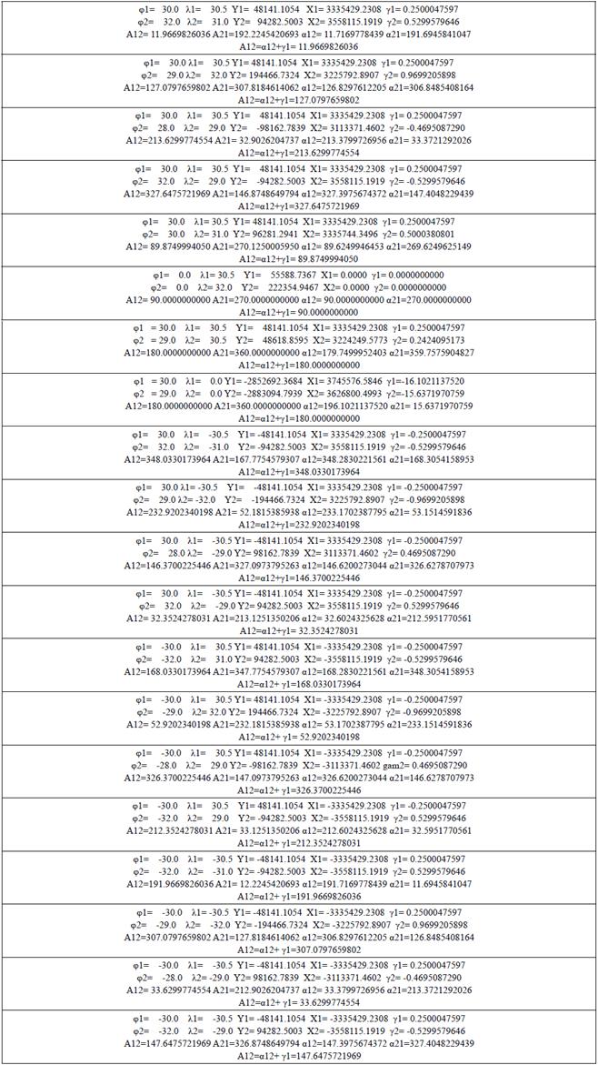
4. Numerical Example
In order to show the validity of the given formulas, numerical applications were made separately in the east and west of Greenwich in both the northern and southern hemispheres. Inverse problem was solved between twenty-point pairs in total. The radius of the earth is taken as R=6370000m, the prime meridian is taken as λprime. =30o to the east of Greenwich and λprime = -30o to the west of Greenwich. In numerical applications (Y, X) Soldner coordinates and (γ) meridian convergences of twenty-point pairs are calculated whose (φ, λ) geographic coordinates are given. Then, the bearing (α) and the azimuth angles (A) calculations were made separately with direct formulas. In order to control between the bearing and azimuth angles, the azimuth angle was found by adding the meridian convergence to the bearing angle (Aijαij +yi) between each pair of points. Numerical application results can be seen in Table 3.
5. Results and discussion
In this study, formulas are given for how to obtain the bearing and the azimuth angle directly without any examination. The numerical examples also show no loss of precision in the use of direct formulas. It has been observed that the classical formulas (Equations 1, 2, 14, and 15) and the formulas we propose (Equations 6, 7, 20, and 21) give the same results in the calculations made with ten digits after the decimal point. It is suggested to use Equations 8, 9, 22, and 23) to avoid division by zero error. The advantage of the method is that no examination is required. In computer calculations, if..., then..., end..., blocks are not used when direct formulas are used. The if..., then..., end..., blocks reduce the execution speed in computer calculations.
The classical formulas and the direct formulas we proposed were compared in terms of processing time. All were coded in MATLAB. The main characteristics of the hardware were Windows 10 Pro, Intel(R) Core(TM) i5-2450M CPU @ 2.50GHz, 6 GB of RAM.
The same bearing and the same azimuth angle were calculated 500 million times and the processing times are shown in Table 4 below.
Table 4 Processing Time
| Bearing Angle | Azimuth Angle | |
|---|---|---|
| Classic formulas | 4.642 sec Eq. 14-Eq. 15 | 5.492 sec Eq. 1-Eq. 2 |
| Proposed formulas | 4.445 sec Eq. 20-Eq. 21 | 4.413 sec Eq. 6-Eq. 7 |
It has been observed that the processing time is slightly shorter in the direct formulas we recommend. This is because classical formulas need quadrant comparison.
6. Conclusion
In this proposed method, formulas are given for how to obtain the bearing and azimuth angle directly without any examination. The need for comparison in classical formulas increases both the processing time and the possibility of error. Direct formulas are always more useful. While saving time on the one hand, the probability of making mistakes will also be seriously reduced on the other hand. We hope that the accuracy and non-examination of the direct formulas we proposed will increase the usability of our formulas. The formulas on the sphere surface, which are used to calculate the direct bearing and azimuth, can also be adapted to the ellipsoid surface. For future studies, researchers are advised to find more simple direct formulas.

