


 Inglés (pdf)
 Articulo en XML
 Referencias del artículo
 Enviar articulo por email
 Citado por SciELO
  Citado por Google
  Similares en
SciELO
Similares en
SciELO  Similares en Google
 Permalink
1. Introduction
Until recently, the oceans have been represented as a single large body with no large-scale temporal variability. Indeed, temporal variability represents an additional difficulty when analyzing features of the ocean, such as eddies, currents, water masses, and primary production. Sea-surface temperature (SST), for example, has been observed by satellites such as those of the series NOAA (National Oceanic and Atmospheric Administration).
Measuring SST is important as it is used in the study of oceanic physical processes such as frontal movements, water masses, currents, and upwelling zones (Barret, 2013; Khan et al., 2021). The present work intends to explore the SST of the tropical Indian Ocean as a major supplement to the more traditional procedures, and to examine the contribution made to an understanding of ocean circulation and water masses at the surface in this region.
Water masses also exist in the surface layer of the ocean. The definition of these water masses in terms of hydrographic properties is not an easy task because they undergo large seasonal and interannual variations. Furthermore, surface water characteristics differ distinctly from one oceanic region to another. Therefore, knowledge of surface ocean temperature can be important in helping to define water masses at the surface.
A water mass which originates at the surface of the ocean is always a result of dynamic interactions between sea and atmosphere. Since a sub-surface water mass usually originates from a well-defined formation region, it is important to know in detail which processes are involved in the water mass formation. Physical and biological properties of surface waters, such as temperature, are constantly changing because of atmospheric and oceanic seasonal variations (Khan et al., 2021). The proximity of land can also be an important factor affecting water masses characteristics, especially if there is a freshwater output from river runoff, such as the Ganges-Brahmaputra-Meghna River catchment in the northern Bay of Bengal (Wang et al., 2022).
The identification and representation of the physical processes responsible for temperature distribution are important steps towards the understanding and management of marine ecosystems. The present study attempts to understand the relationship between regional circulation and the variability of temperature and its distribution at the surface of the Indian Ocean. Long-term analysis of SST can be particularly useful to describe the main mechanisms that operate at the surface of the ocean, such as formation of water masses at the surface.
The study of temperature in the oceans play a major role in the analysis of global warming. The interaction between atmosphere and SST is important to monitor and predict climate change (Wang et al., 2022). The monsoon regime of the Indian Ocean, for example, is highly dependent on the SST (Alory et al., 2007; Huang et al., 2021; Liao and Wang, 2021; Khan et al., 2021). Khan et al (2021), define a four stages cycle for the SST in the tropical Indian Ocean, with a warming stage from February to May, a cooling from May to August, warming again from August to October and another cooling from October to January.
Two main regions can be distinguished in the Indian Ocean, the northern and the southern Indian Ocean (McPhaden, 1982; Tomczak and Godfrey, 1994). The northern Indian Ocean comprises three regions: the equatorial Region (10° N to 10° S), Bay of Bengal and Arabian Sea. The great seasonal changes observed in the northern Indian Ocean are commonly attributed to the presence of the Eurasian land mass and the absence of temperate and polar regions (Shetye et al., 1994; Singh and Roxy, 2022). These result in a strong seasonal difference in the distribution of centers of pressure, which originates the monsoons. The boundary of the southern Indian Ocean to the south is not clear, and some researchers prefer to include the Antarctic Circumpolar Current.
Three general circulation systems are defined to the Indian Ocean: the seasonal monsoon gyre, the subtropical anticyclonic gyre of the Southern Hemisphere, and the Antarctic waters with the circumpolar current (Wyrtki, 1973; Reid, 2003; Naqvi, 2008) (Figure 1). The fact is that it is the seasonal reversal of the monsoonal gyre that gives the Indian Ocean its principal and unique characteristics.
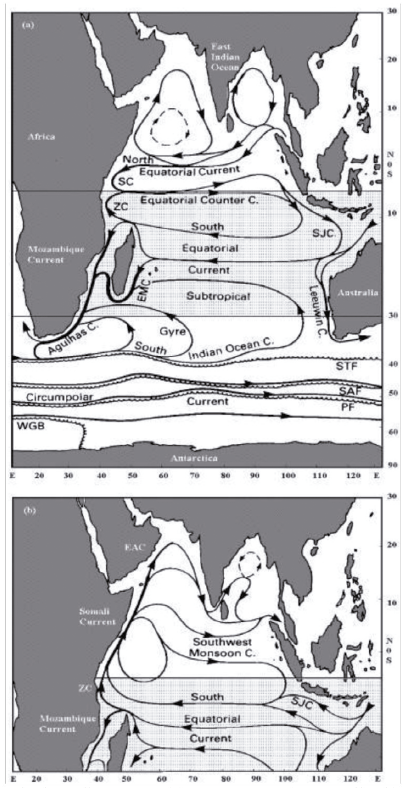
Figure 1 Surface currents in the Indian Ocean. (a) NE Monsoon (Dec-April); (b) SW Monsoon (Jun-Oct). EAC = East Arabian Coast; SJC = South Java Current; ZC = Zanzibar Current; EMC = East Madagascar Current; SC = Somali Currents; STF = Subtropical Front; SAF = Sub-Antarctic Front; PF = Antarctic Polar Front; WGB = Weddell Gyre Boundary. Source: Tomczak and Godfrey (1994).
During the NE Monsoon, the main water flow in the equatorial region of the Northern Hemisphere is from east to west. North Equatorial Current turns southwards along the Somali coast and, together with the Zanzibar Current, flows Eastwards on both sides of the equator (Equatorial Counter Current). Some water from the Equatorial Counter Current returns as the South Equatorial Current (Zanzibar Current) while the residue travels southeast as the Java Current (Schott and McCreary, 2001; Semba et al., 2019; Jacobs et al., 2020).
The SW Monsoon starts in April with a northward flow along the Somali coast. Already in May, an eastward flow is well pronounced north of the equator. Around July, the Somali Current becomes stronger and the counter current at the equator is replaced by the SW Monsoon Current. Below the equator, the South Equatorial Current, coming from the east, turns north along the African coast and becomes the Somali Current (Tomczak and Godfrey, 1994). This current has an important effect on the local baroclinic adjustment.
This work describes the temperature distribution in the surface layer of the tropical Indian Ocean (25° N to 30°S and 30° E to 120° E) based on analysis of semiannual and annual amplitudes of temperature and a multiple regression analysis between temperature, Ekman pumping, components of pseudo-stress wind, wind magnitude and NDFF. It is expected that this study can contribute to the definition of water masses on the surface of the Indian Ocean.
A long-term data set is explored to a large-scale examination of the SST of the tropical Indian Ocean as a major supplement to the more traditional procedures, and to examine the contribution made to an understanding of ocean circulation in this region. The process aims to examine how the two components of the harmonic fit contribute and interact to produce the observed and modelled data cycle.
2. Data and methodology
A set of five degree by five-degree grid average monthly SST contour plots for the Indian Ocean is produced based on the World Ocean Atlas Data Set (1994). The aim is to use the AVHRR MCSST/NOAA satellite data to estimate a matrix, which will be then matched to another matrix originated for the World Ocean Atlas Data Set. All the temperature data are thus arranged on a five-degree latitude-longitude grid, only for the surface of the oceans (zero meter) with a final spatial resolution of 500 km2.
Temperature, wind, NDFF, and Ekman pumping are included in a multiple regression analysis to define the relative importance of each one of these variables in the physical processes at the surface of the Indian Ocean. The NDFF data set is based on COADS (Comprehensive Ocean-Atmosphere Data Set) and obtained from Oberhuber (1988). It is originally organized in a 2° X 2° grid and averaged in 5° x 5° grid for this research. The NDFF represents the balance between precipitation and evaporation, with a unit of mm.
The wind data is obtained from the Florida State University (FSU) Wind Stress Data Set for the tropical Indian Ocean in a 1° x1° grid. The data is averaged in a 5° x 5° grid. The FSU data set is based on COADS and NCEI (National Centers for Environmental Information). The wind stress is presented as pseudo-stress wind, which is the wind component multiplied by the wind speed, at a reference height of 10 m.
For temperature, the twelve-monthly mean values are subjected to a harmonic analysis to determine the two harmonic components, one having a period of one year and the other a period of six months. The process aims to examine how the two components contribute and interact to produce the more complex cycle of the observed and modelled data.
The harmonic terms are considered to be stationary, as the averages and corresponding autocorrelations are not expected to vary significantly in a long period of time. The Fourier series for the stationary time series of temperature can then be expressed symbolically as a cosine function, in which the first and second harmonic terms are multiplied by the maximum amplitude of the variable and added to the mean annual parameter.
The modelled data can thus be expressed as: O(t) = Ō + A x cos (ω α xt-a) + B x cos (ω s x t - b) (Katznelson. 2004), where: O(t) = observed value as a function of time when t is time in days, since the start of an arbitrary year, Ō = mean value over the period analyzed, A = Amplitude of the annual harmonic component, B = Amplitude of the semiannual harmonic component, α = Phase-lag of the annual component, b = Phase-lag of the semiannual component, ω = Angular frequency (2 π /365.25), which represents the increment in phase per unit time, t, of the annual harmonic component, ω s = ditto for the semiannual component but (2π/182.62), (ω x t-α) = phase of the annual harmonic, (ω xt - b) = phase of the semiannual harmonic.
Values of O, A, B, a and b are to be determined by analysis. They represent the average annual temperature and are a positive constant. The amplitude value (A or B) is also a positive constant that represents the amplitude of the motion and so its maximum departure from the mean value as the term oscillates within a range of + or -. Phase-lag is expressed in degrees, with 30° per month for the first harmonic and 60° per month for the second. Phase-zero implies that a maximum occurs at the mid of January. It expresses the average time when the maximum of SST occurs within the annual cycle. For example, the phase of 120° corresponds to the mid of April, 150° to the mid of May, and 270° to the mid of October.
The sum of square residual is defined as: SSres = ∑ (Y - Y') 2 and represents the sum of squared differences between observed (Y) and the predicted values (Y'), these differences representing the small inadequacies of the fit. R-squared describes how well the temperature is explained by the combination of the independent variables as a single unit and is expressed as percentage. R squared ranges between 0 and 1 and is represented by R2=1-SSres/SS total, where SSres is the sum of the squares of the residuals and SS total is the total sum of the errors. The closer to one the better. Therefore, R-squared is the percent of variance explained by the temperature model. In other words, R-squared is the fraction by which the variance of the errors is less than the variance of the dependent variable.
3. Results
The 5° x 5° grid average SST contour plots during the SW Monsoon (July, August, and September) can be seen in Figure 2. In the northern Indian Ocean, the isotherms are mainly meridional along the western boundary, within the range of the Somali Current which runs from south to north during the SW Monsoon.
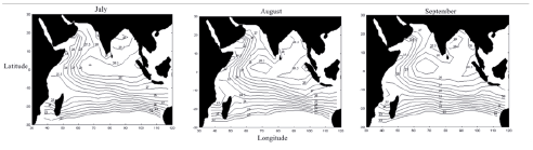
Data Source: World Ocean Atlas Data Set (1994).
Figure 2 Average SST (°C) based on a 5° x 5° degrees grid for the SW Monsoon (July, August, and September).
A zonal distribution of temperature is observed in the southern Indian Ocean, and a tongue of high temperatures above 28 °C is present along the equator and east of 60° E. The influence of the tongue extends northwards into the Bay of Bengal and west of India, as can be seen from the 28 °C and 28.5 °C isotherms. High temperatures, close to 29 °C, are observed in the north Bay of Bengal. The upwelling areas along the Somali and Arabian coasts are marked by temperatures below 26 °C. The isotherms in the western region of the southern Indian Ocean, around Madagascar, deflect slightly northwards and southward because of the South Equatorial Current, which runs from east to west and splits into two branches in this area.
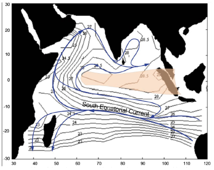
Figure 3 is a graphic representation that relates Figure 1 and Figure 2, superimposing the regional circulation of the Indian Ocean with the distribution of isotherms. The objective is to provide a synoptic view of the study area, highlighting the importance of SST in the physical processes related to the monsoon regime. As can be seen, the isotherms reliably represent most of the oceanographic features in the study area, as the South Equatorial Current, which can be associated with the intensification of the zonal temperature gradient in the region. Warm water from the Pacific into the Indian Ocean is highlighted in yellow.
The distribution of SST contours on a 5° x 5° grid average for January, February, and March, during the NE Monsoon, can be observed in Figure 4. During this time of the year, the circulation of the area is dominated by the North and South Equatorial Currents, as a consequence of the westerly winds blowing along the equatorial belt. Since the northeast trades are strong because of the high-pressure system established in the Asiatic region, temperature contours tend to be meridional (south-northeast direction) north of the equator.
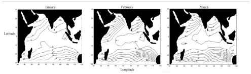
Figure 4 Average SST (°C) based on a 5° x 5° grid for the NE Monsoon (January, February and March). Data Source: World Ocean Atlas Data Set (1994).
Figure 5, like Figure 3, is a graphic representation that associates Figure 1 and Figure 4, superimposing the regional circulation of the Indian Ocean with the distribution of isotherms during the NE Monsoon. It is also clear to see the warm water tongue coming from the Pacific, shown in yellow.
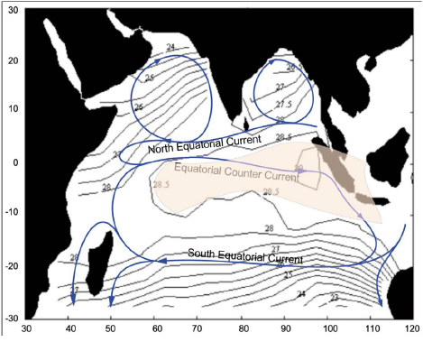
Figure 5 Superposition of the main currents and isotherms in NE Monsoon, with reference to the month of February.
Comparing Figures 3 and 5, it is clear that the main features, such as the South Equatorial Current and the meridional isotherms in the Persian Gulf, are present. The difference is in the intensity. Temperature along the west coast of the Indian Ocean during the NE Monsoon is more uniform, varying from 26 to 28 °C, and no strong temperature gradients are observed in the region along the Somali and Arabian coasts. Below 10° S, the isotherms deflect slightly southward in the coastal areas of the southern Indian Ocean, Madagascar, and the Australian coast.
There are two main currents in this region: the South Equatorial Current and the Subtropical Gyre. These result in an anticyclonic circulation with a mainly westward direction between 60° E and 100° E. To the west, the flow is southward and along the Madagascar coast. In the eastern Indian Ocean, close to Australia, the surface circulation is initially southward, before switching to a westward direction. The influence of these major circulation systems is seen in the curved shape of the temperature contours.
The temperature variation through an average year, as expressed through the amplitude of the annual (first) and semiannual (second) harmonic, can be seen in Figure 6. The smallest amplitude values of the annual and semiannual components (below 0.5 °C) are found along the equator, especially in the eastern part. Here, the SST exceeds 28 °C throughout the year (Figures 6a and 6c). The largest amplitude values are found in the western Indian Ocean, the Arabian Sea, the Bay of Bengal, and south of 20° S. Figures 6b and 6d show the phase lags for the first and second harmonics of the SST.
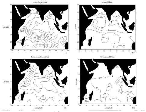
Figure 6 (a) Distribution of SST amplitude for the first harmonic. (b) Distribution of SST phase-lag for the first harmonic. (c) Distribution of SST amplitude for the second harmonic. (d) Distribution of SST phase-lag for the second harmonic. Annual and semiannual amplitudes of SST are expressed in °C. Amplitude and Phase of temperature are calculated from the World Ocean Atlas Data Set (1994).
Phase-lag is expressed in degrees and increments at 30° per month for the first harmonic and 60° per month for the second, where phase is zero it implies that a maximum occurs in mid-January. It expresses the average time when the maximum of SST occurs within the annual cycle. For example, phase of 120° corresponds to mid of April, 150° mid of May and 270° mid of October. They indicate the time of the year when the maximum amplitude occurs.
Figure 7a shows the observed data and the two harmonic components fit to the observations. Figure 7b shows the two individual harmonic components and their interaction through the year in the Arabian Sea. The annual component is seen to have a maximum in July (SW Monsoon) and a minimum in January (NE Monsoon) which suggests a connection with a hot summer and a cold winter, likely due to proximity to a continental land mass in these latitudes. Compared with the annual component, the amplitude of the semiannual component is smaller, with two maxima in May and October and two minima in February and August (Figure 7b). A similar pattern is observed in the Bay of Bengal, but the two maxima (April and October) and the two minima (January and July) occur earlier than in the Arabian Sea.
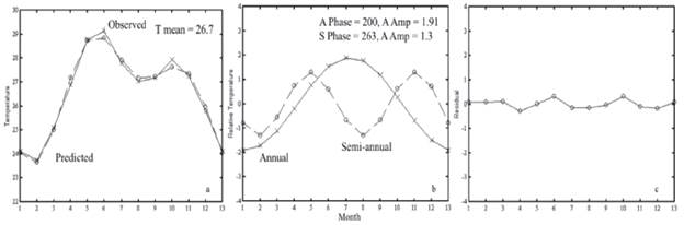
Figure 7 (a) Observed and two components fit to observations (°C). (b) First and second components of the harmonic analysis. (c) Residual plot between observed and harmonic temperature (°C). Time (months) in which 13 is equal to 1 and corresponds to mid-January of the following year.
The overall fit is good, with a residual sum of squares of 0.39. In fact, the residual errors between observed and harmonic temperature are small, with a maximum of 0.32°C during June (Figure 7c). The small magnitude of these residuals suggests that the temperature variability during this period and for this particular area can be explained reasonably well by just the two harmonic terms.
The sum of square residual can be defined as SSres = ∑ (Y - Y')2 and represents the sum of squared differences between observed (Y) and the predicted values (Y') These differences represent the small inadequacies of the fit. McPhaden (1982) applied residual variance from regression techniques to analyze equatorial waves in the Indian Ocean. Another study based on correlations between amplitudes and phases used a wind-driven model for the North Pacific (White, 1978).
Figure 8 compares the observed and two components harmonic fit of the Somali coast (52.5° E and 7.5° N) sea surface temperature (SST), the annual and semiannual components, and the residual errors. The highest annual component occurs in March/April. During this period, the area is affected by the North Equatorial Current and the anticyclonic flow, which are responsible for the input and re-circulation of warm equatorial waters into the Arabian Sea. The minimum of the annual component occurs in September/October, when the Somali Current represents the strong northward flow observed along the western Arabian Sea (Figure 8a).
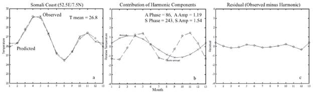
Figure 8 (a) Observed and two components fit to observations (°C). (b) First and second components of the harmonic analysis. (c) Residual plot between observed and harmonic temperature (°C). Time (months) in which 13 is equal to 1 and corresponds to mid-January of the following year.
The two peaks of the semiannual component occur in April/May and October/November, transition months between the monsoons, when wind stress is weaker and less evaporative cooling and mixing are expected (Figure 8b). These result in the high temperature observed during April and May. The two minima occur in January/February and July/August. The first is associated with the peak of the NE Monsoon and a slight winter cooling. The increase in wind speed, which results in large evaporative cooling and mixing, can explain the secondary low peak of temperature during this period.
The second minimum that occurs during July/August can be explained by the strong wind stress and upwelling that occurs during this time of the year. Since the annual and semiannual components are acting almost in conjunction, it is expected that the wind monsoon drive circulation is also contributing to this peak of low temperature. The semiannual (-1.4) and annual (-0.86) signals are both strong during August. The low residual errors (maximum of 0.38 °C in January) show a good agreement between observed and the two components harmonic fit, with a residual sum of squares of 0.4 (Figure 8c).
Figure 9a compares the observed SST with the two components harmonic fit at a position on the equator, 62.5° E and 2.5° S. It is possible to see how the harmonic contribution due to the interaction between the annual and semiannual components affects the two harmonic components fit (Figure 9b). The maximum of the annual component occurs in April and the minimum in October, which suggests that the variability of solar radiation is connected to this. The two maxima of the semiannual component are observed for April/May and October/November, the transition between the monsoons. The low residual errors indicate a good agreement between observed and the two components harmonic fit (Figure 9c).
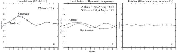
Figure 9 (a) Observed and two components fit to observations (°C). (b) First and second components of the harmonic analysis. (c) Residual plot between observed and harmonic temperature (°C). Time (months) in which 13 is equal to 1 and corresponds to mid-January of the following year.
The final regression equations for temperature variability in the Arabian Sea show that temperature is mainly affected by the Wx, Ekman pumping and NDFF (Table 1). Components of wind stress, wind magnitude, Ekman pumping and NDFF are impacting the temperature, but the Wx is a constant presence in all of the equations.
Table 1 Predicted equations for the eastern Arabian Sea.
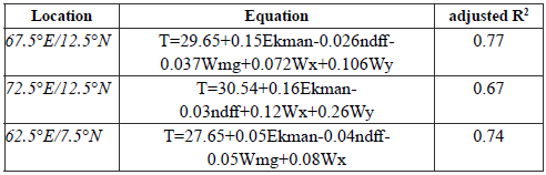
Wx = zonal component of pseudo-stress wind (m 2 s -2 ), Wy = meridional component of pseudo-stress wind (m 2 s -2 ), NDFF = net-down-fresh-water-flux (mm), Ekman pumping = (-) downward/(+) upward (xl0 -3 kg.m 2 .s -1 ), T = temperature (°C), Wmg = wind magnitude (ms -1 ).
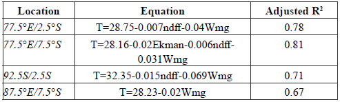
The final regression equations and their respective adjusted R-squared values for the Bay of Bengal are shown in Table 2. For most of the areas of the Bay of Bengal, temperature can be explained by the entered independent variables. The meridional component of the wind stress (Wy) is one of the main variables that affects temperature. All final regression equations have larger values of beta coefficients for this variable. It is followed by the zonal components of the wind stress (Wx) and NDFF, in order of importance.
Table 2 Predicted equations for temperature at the Bay of Bengal.
Wx = zonal component of pseudo-stress wind (m 2 s -2 ), Wy = meridional component of pseudo-stress wind (m 2 s 2 ), NDFF = net-down-fresh-water-flux (mm), Ekman pumping = (-) downward/(+) upward (x10 -3 kg.m 2 .s -1 ), T = temperature (°C), Wmg = wind magnitude (ms-1).
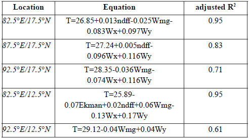
The final regression equations for temperature at the equatorial region, with an adjusted R-squared greater than 0.6, can be seen in Table 3. The temperature in these areas can be explained by the independent variables. The magnitude of the wind and NDFF are the main variables responsible for the temperature variability.
Table 3 Predicted equations for the equatorial region (60° E to 100° E and 10° S to 5° N).
Wx = zonal component of pseudo-stress wind (m 2 s -2 ), Wy = meridional component of pseudo-stress wind (m 2 s 2 ), NDFF = net-down-fresh-water-flux (mm), Ekman pumping = (-) downward/(+) upward (x10 -3 kg.m 2 .s -1 ), T = temperature (°C) and Wmg = wind magnitude (ms -1 ).
A set of final regression equations for temperature in the southern tropical Indian Ocean region with an adjusted R-squared larger than 0.6 is shown in Table 4. These equations demonstrate that the variables affecting the temperature vary significantly from one location to another. Temperature can be predicted for most of the locations, but the independent variables vary significantly from one location to another. For the locations at 57.5° E/17.5° S, 72.5° E/22.5° S, 87.5° E/17.5° S and 57.5° E/27.5° S, temperature can be predicted from only one independent variable at each location, NDFF, Ekman pumping, Wy, and Ekman pumping, respectively. The largest Beta coefficients are obtained for Wy, Ekman pumping and NDFF.
Table 4 Predicted equations for the south tropical Indian Ocean (30° S to 10° S).
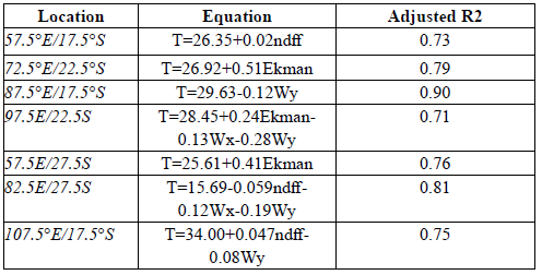
Wx = zonal component of pseudo-stress wind (m 2 s -2 ), Wy = meridional component of pseudo-stress wind (m 2 s 2 ), NDFF = net-down-fresh-water-flux (mm), Ekman pumping = (-) downward/(+) upward (x10 -3 kg.m 2 .s -1 ), T = temperature (°C) and Wmg = wind magnitude (ms -1 ).
4. Discussion
The amplitudes of the annual component increase with latitude in the north Indian Ocean and reach maximum values to the north of the Arabian Sea and Bay of Bengal. This distribution reflects the response of the ocean to the solar radiation, in which amplitudes increase away from the equator. The reversal of the monsoons, associated with land mass distribution also results in a large contribution to these large amplitudes. The latest occurrence of the annual maximum temperature is observed in the northernmost parts of the Arabian Sea and Bay of Bengal, where the maximum of the annual occurs in July.
The importance of the solar path is clear in the annual component of temperature, but it also seems that the boundaries have an influence on winter temperatures north of the Arabian Sea and Bay of Bengal. It is believed that larger amplitudes result from colder winters over adjacent continental land, due to the contrast between cold air and warmer sea surface water.
The maximum semiannual amplitude observed for May and October are associated with the transition months between the SW Monsoon and the NE Monsoon. During May and October, wind intensity is expected to decrease, which would reduce evaporative cooling and water mixing. This could explain the raise in temperature during these periods. It also seems that the two minima, observed during February and August, can be linked to the peaks of the NE Monsoon and SW Monsoon, respectively. Winter cooling (in the case of the NE Monsoon) associated with maximum wind during these periods can result in large evaporative cooling and stirring of the water, which can decrease the SST. This is in line with Khan et al. (2021) when studying the monthly cycle of SST in the North Arabian Sea for 2016/2017, from Satellite and Argo datasets.
The interaction between the annual and the semiannual component of SST results in a depression of the temperature from mid-July to mid-September when the large annual peak of the annual component (summer leading to large solar radiation) act in opposition to the small negative peaks of the semiannual component (wind stress leading to large evaporation and mixing). The pronounced low temperature observed during February could be due to the annual component (low solar radiation during winter) working together with the semiannual component (strong wind, leading to large evaporation and mixing).
In the Indian Ocean, the amplitude of the semiannual component can be comparable to the annual component. In some regions, such as the Somali (47.5° E and 7.5° N) and Arabian coast (52.5° E and 12.5° N), the semiannual component is considerable larger than the first harmonic with maximum amplitudes around 1.6 °C. The strong semiannual component along the Somali and Arabian coasts is thought to be associated with coastal upwelling derived from the strong monsoonal wind field acting upon a left-hand coastline from June to October. This semiannual variability of temperature is influenced by wind, since large values of semiannual periodicity also occurs in the western Arabian Sea (Unnikrishnan et al., 1997; Khan et al., 2021). Previous works, such as that of Levitus (1987) and Khan et al. (2021) have already demonstrated semiannual cycles of temperature in the Indian Ocean. These cycles could be related to evaporative cooling and upwelling associated with the monsoons.
The two maximum values of the semiannual component, seen in April/ May and October/November, are a result of the weaker wind stress during these periods, when less evaporative cooling and mixing are expected. These result in the high temperature observed during April and May. The first semiannual minima, observed in January/February and July/August, is associated with the peak of the NE Monsoon and a slight winter cooling.
The increase in wind magnitude, which results in large evaporative cooling and mixing, can explain the secondary low peak of temperature during this period. The second minimum that occurs during July and August can be explained by the strong wind stress and upwelling that occur during this time of the year. It is expected that the wind monsoon drive circulation is also contributing to this peak of low temperature, since the annual and semiannual components are acting almost in conjunction.
One of the main characteristics of the equatorial Indian Ocean is its lack of upwelling. As a result of the dominance of the meridional orientation of the wind, Ekman transport does not result in divergence along the equatorial region and, therefore, no upwelling occurs (Tomczak and Godfrey, 1994). However, the overall pattern with a secondary low during August remains, even where no upwelling is expected. The low will be located along the equatorial region, away from the coast and west of 70° E.
The two maxima of the semiannual component, observed in April/ May and October/November, can be associated with weaker winds during these months, which result in less evaporative cooling and mixing. The larger temperature value for April can be attributed to the fact that the annual component acts with the semiannual component, and the opposite for October/ November. For example, during October and November, the annual (negative) and semiannual (positive) components act in opposition.
The semiannual component (0.37 for October and November) is similar in magnitude to the annual but opposite in sign (-0.58 for October and -0.51 for November) and results in the secondary high-temperature peak observed during these months. The annual and semi-annual components, acting together from March to June, enhance the temperature during this period, with a maximum temperature peak during April. The distribution of the residual between the observed and the two harmonic fit reveals that the harmonic model is meaningful, as the maximum residuals are observed from February to May and are below 0.12 °C.
In fact, only to the west of 70° E along the equator is the second harmonic temperature larger than 0.5 °C, with the two maxima occurring during April and November. The amplitude becomes weak eastward, along the equator, and, therefore, the seasonal variations are considered to be insignificant in this area. The low amplitude values east of 70° E are a result of an expected low rate of exchange between ocean and atmosphere near the equator, for example the lack of wind when compared to the higher latitudes.
In the Southern Hemisphere, the maximum amplitude of temperature of the annual component occurs late January along the south coast of Africa. The annual component increases eastwards, reaching a maximum during early March in Australia. The annual component increases gradually towards the north, following the solar path, as shown by the phase-lag distribution. A gradual phase-lag shift (30° to 130°) from the southern to Northern Hemisphere is observed in the tropical region from 10° S.
5. Conclusion
Large annual variations in temperature were observed in the north of the Arabian Sea and Bay of Bengal, in the western equatorial region and in the southern tropical Indian Ocean. Large semiannual fluctuations in temperature were observed along the western boundary of the Indian Ocean, from 10° S to 25° N. Based on multiple regression analysis, it was possible to identify and quantify the variability of the temperature. For example, the temperature within upwelling regions along the Somali and Arabian coasts could be explained by the variability of the components of the pseudostress wind, wind magnitude and Ekman pumping, with an adjusted R-squared ranging from 0.64 to 0.84.
The annual component, overall, is related to large-scale features of the seasonal solar radiation input and the seasonal monsoons. Basic features associated with the monsoons, such as wind-driven advection, can have a significant influence on the annual term. The semiannual component is influenced by local and regional factors, which add to the basic pattern defined by the annual term. These local and regional influences are the result of different processes, such as upwelling and the non-directional effect of wind stress (e.g., evaporation, precipitation, and mixing).
This study is expected to contribute to the understanding of the Indian Ocean, especially regarding the processes involved in the interface between the atmosphere and the ocean surface. This understanding may also contribute to the study of the water masses at the surface of the Indian Ocean and their expected impacts on climate change in the region.

