Detection of Fraudulent Transactions Through a Generalized Mixed Linear Models

Gómez-Restrepo, Jackelyne; Cogollo-Flórez, Myladis R

Services on Demand

Journal

Article

Indicators

Cited by SciELO
Access statistics

Ingeniería y Ciencia

Print version ISSN 1794-9165

ing.cienc. vol.8 no.16 Medellín July/Dec. 2012

ARTÍCULO ORIGINAL

Detection of Fraudulent Transactions Through a Generalized Mixed Linear Models

Detección de transacciones fraudulentas a través de un Modelo Lineal Mixto Generalizado

Jackelyne Gómez-Restrepo¹ y Myladis R. Cogollo-Flórez²

¹ Mathematical Engineer, jgomezr7@eafit.edu.co, Masters student, Universidad EAFIT Medellín-Colombia.

² Master in Science in Statistics, Ph.D.(C) Systems and computer Engineering, mcogollo@eafit.edu.co, professor, Universidad EAFIT, Medellín-Colombia.

Received:17-feb-2012, Acepted: 18-oct-2012Available online: 30-nov-2012

MSC:62p05

Abstract

The detection of bank frauds is a topic which many financial sector companies have invested time and resources into. However, finding patterns in the methodologies used to commit fraud in banks is a job that primarily involves intimate knowledge of customer behavior, with the idea of isolating those transactions which do not correspond to what the client usually does. Thus, the solutions proposed in literature tend to focus on identifying outliers or groups, but fail to analyse each client or forecast fraud. This paper evaluates the implementation of a generalized linear model to detect fraud. With this model, unlike conventional methods, we consider the heterogeneity of customers. We not only generate a global model, but also a model for each customer which describes the behavior of each one according to their transactional history and previously detected fraudulent transactions. In particular, a mixed logistic model is used to estimate the probability that a transaction is fraudulent, using information that has been taken by the banking systems in different moments of time.

Key words: Generalized linear model, transactional history, detected frauds, outliers detection.

Resumen

La detección de fraudes ha sido uno de los temas en el que muchas compañías del sector financiero han invertido más tiempo y recursos con el fin de mitigarlo y de esta forma mantenerse a salvo; sin embargo, encontrar patrones dentro de las metodologías empleadas para cometer fraude en entidades bancarias es un trabajo que involucra ante todo conocer muy bien el comportamiento del individuo, con la idea de finalmente hallar dentro de todas sus transacciones aquellas que no corresponderían a lo que habitualmente éste hace. De esta forma, las soluciones planteadas hasta la fecha, para este problema se han trasladado únicamente a poder identificar outliers o datos atípicos dentro de la muestra que se está analizando, lo cual no permite analizar cada individuo de manera individual y mucho menos realizar un pronóstico de fraudes. En este trabajo se evalúa el uso de un modelo logístico mixto para la detección de fraudes. Este modelo, a diferencia de los métodos convencionales para detección de fraudes, considera la variabilidad de las transacciones realizadas por cada individuo; lo que permite generar no sólo un modelo global, sino también un modelo por cada individuo que permite estimar la probabilidad de que una transacción realizada sea fraudulenta, teniendo en cuenta su historial de transacciones y las transacciones fraudulentas detectadas previamente.

Palabras claves: Modelo lineal generalizado, historia transaccional, fraudes detectados, detección de outliers.

1 Introduction

Among the methodologies used for detecting fraud through magnetic strip cards, are those used to detect patterns or anomalies, that determine a fraudulent action as an event which is not consistent with others, in this way it takes using data mining tools which use statistics science, optimization and large volumes of information. [1], since 1997 to 2008, perform a review of the state of art about applications of data mining in financial fraud detection. They find that most common data mining techniques applied to detect fraud are methods of classification [2],[3],[4],[5] and clustering [6],[7],[8]. In [9],[10] the authors review the statistical techniques used for detecting fraud. Specifically, the most used methodology, for fraud detection through magnetic stripe cards, is linear discriminant analysis. Similarly, artificial neural networks (ANN) are used for forecasting this kind of behaviour; in [7] propose an unsupervised neural network for detecting and creating criteria to identify suspicious individual behaviours, using trends and characteristics of individuals. Meanwhile, in [11] proposed a supervised network, using 3 hidden layers and back-propagation algorithm to determine patterns of fraud. In [12] makes a comparative research among an ANN, decision trees and Bayesian networks. With decision trees, branches could gather almost every abnormal movement, but this kind of model requires an initial analysis of the variables to determine whether or not independent. The method that worked better was ANN, followed by the decision tree, and finally Bayesian network. Besides, about the variables that should be used for detecting fraud, [13] proposed a detailed research for choosing correctly variables and methodology, they suggest using amount, type (payment, check, etc.), type of market in which it was used, channel and check mode (PIN or chip or magnetic stripe). Also they proposed to use aggregated information from each individual in order to have all history available, and thereby make predictions of the behaviour of each person, and when a transaction gets an abnormal patter it will be considered as an alert to analyse. In many cases, be an expert minimizes the work to select a methodology and leads to create hard rules that not determine all abnormal movements, but mostly of them; in [14] are applied different rules for gain knowledge of patterns of individual transactions. However, as mentioned, this methodology involves having a vast knowledge of the individual and the system, as they must create rules based on the history to create implications that would be used as a criterion for determining whether conduct is suspected or not (fuzzy logic).

Generally, in the literature there are proposals made for fraud detection through magnetic stripe cards, which are based on classification and clustering techniques or ANN, in which individuals are classified according to general rules. These techniques assume that individuals have a similar variability, a common pattern, and they do not examine individual variability for each client in their financial transactions. This is a disadvantage and may lead to problems in the quality of detection because not all individuals operate equal; in real life each individual has a unique behaviour that should be studied as such. This paper proposes the use of a mixed logistic model to determine suspicious transactions through transactional information of individuals. As well as estimating fraud within the organization, the model determines a model for each client, taking into account individual behaviour.

This paper is divided into five sections, first one describes an overview about theory of linear mixed models, the second part has information about theory of generalized linear mixed models, the mixed logistic model is considered as a particular case, third section presents the use of mixed logistic model to detect fraud, and finally conclusions and references are presented.

2 General Linear Model with Mixed Effects

Linear mixed models have been increasing their popularity in applied statistics literature for health sciences, because they represent a powerful tool to analyse data with repeated measures, frequently obtained in studies of this area. The existence of repeated measurements requires special attention to the characterization of random variation in data. In particular, it is important to explicitly recognize two levels of variability: random variation between measures within a particular individual (intra-individual variation) and random variation between individuals (inter-individual variation). The linear mixed model considers these sources of variation and can be defined by the following two steps:

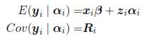
Step 1: Modelling intra-individual variation. Suppose that for the i-th of m individuals, ni responses have been observed and that a total of N = n_i data are available. Let be y_i the vector of responses for the individual i-th, which satisfies

where β is a vector of parameters (p x 1) that corresponds to the fixed effects, x_i is a matrix for the i-th individual which characterizes the systematic part of the answer; α_i is a vector (k x 1) characteristic of the i-th individual, z_i is a design matrix (n_i x k) and e_i is the vector of intra-individual errors. Assumes that e_i N_ni(0,R_i), where R_i is a covariance matrix intra-individual of size (n_i x n_i). So, from model (1):

Step 2: Modelling inter-individual variation.

Suppose that the vector of random effects α_i is obtained from a normal distribution with mean zero and dispersion matrix D(_{k x k}); besides assume that α_i; i = 1, ... ,m, are mutually independent. So, under these assumptions:

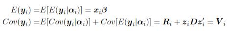
That is, the model (1) with the above assumptions for e_i and α_i implies that y_i is a multivariate normal random vector of dimension n_i with a particular form of covariance matrix, it means: y_i N_ni(x_i,β, V_i). The shape of V_i implies that the model has two different components of variability, the first one refers only to the variation within individuals (R_i) and the second one refers to the variation between individuals (D). In the adjustment process of a mixed model is common to consider three components: the estimation of fixed effects (β), the estimation of random effects (α_i) and the estimation of covariance parameters (D y R_i)[15]. The standard approach under the multivariate normality assumption is to use the method of maximum likelihood (ML) and restricted maximum likelihood (REML). Although Bayesian concepts are also used to estimate α_i.

The next section will present a brief introduction to generalized linear mixed models, which are extensions of models above but now the response variable is not continuous.

3 Generalized Linear Mixed Model

Generally, linear mixed models have been used in situations where the response variable is continuous. However, in practice there are cases where the response may be a discrete variable or categorical; for example, the number of heart attacks in a potential patient during the last year takes values as 0, 1, 2, ... In these cases, Generalized linear mixed models (GLMM) are used, a GLMM is an extension of the linear mixed model where responses are correlated and can be categorical or discrete variables [16]. To define a GLMM, two stages need to be mentioned:

Stage 1: Select a random sample of n individuals from a population of size N. Attach to the i-th individual an specific parameter αi.

Stage 2: According with αi, select repetitions of [y_ij, x_ij];; i = 1, ..., n,j = 1, ... , n_i. Suppose that per individual, y_ilαi the repetitions are statistically independent, such that:

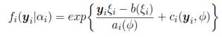
Where b, a, c are known functions, and ψ is the dispersion parameter which may be or may be not known. ξ_i is associated with µ_i = E(y_ilα_i), which is associated with the linear predictor: η_i = α_iz'_i + x_i β through a link function g(.), such that g(µ_i) = η_i. For this case, z_i are registered variables that represent a random effect for the i-th individual. Models as mixed logistic model, mixed Poisson model, Probit model and other can be obtained with different link functions.

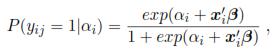
The methodology which was proposed is based on a mixed logistic model; the model was obtained with a sampling scheme of two stage, where y_ilα_i Ber(p_i) is assumed i.i.d., and with p_i = P(y_ij = 1lα_i). Also, the link function is a logit:

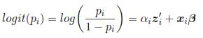
A logistic model with random intercept is obtained if z_ij = 1.

Where α₁, ... , α_n are i.i.d., such that α_i h_α(θ).

Note that this type of model can be extended to case where y_ilα_i Multinomial(p₁,..., p_k). So, the model can predict the likelihood that a subject belongs to one of the k groups. The model's predictive ability is assessed by comparing the observed data and the predicted data; the model classifies individuals in each group defined by the dependent variable based on a cut off point set for the predicted probabilities from the estimated coefficients and the value taken for each explanatory variable. [17].

The interpretation of coefficients and the criteria of goodness of fit are:

i. Theoretical value and interpretation of coefficients.

The shape of the theoretical value in a logit regression is similar to values in a multiple regression, and it represents a unique relationship with coefficients which indicate the relative weight of each predictor. The calculation of a logit coefficient compares the probability of occurrence of an event with the probability that it does not happen. β are measures of changes in the odds ratio [18]. In some cases, the coefficients are logarithmic values, so they should be transformed to do a correct interpretation of them; taking into account that a positive coefficient increases the probability of occurrence while a negative has an opposite effect.

ii. Model evaluation.

Logit models with random intercept, unlike linear models, are not assessed with the R² or through the AIC coefficient, because the methods for calculating them require a high complexity, computation time and perhaps, in many cases, the methods cannot converge. So that, rates and indicators are used to get an idea of model behaviour:

Misclassification rate: Refers to the probability of classifying a 0 as 1 or vice versa.

Good classification rate: Refers to the probability of classifying a 1 as 1 or vice versa.

Specificity: Refers to the probability of classifying a 1 as 1 given that it is 1.

Sensitivity: Refers to the probability of classifying a 0 as 0 given that it is 0.

4 GLMM for detecting fraud transactions

According to the literature, the use of classification and clustering techniques have been proposed for the detection of fraud through swipe cards [2],[3],[4],[5], [6],[7],[8],[9],[10]; but, these techniques just create a classification rule assuming that all individuals have an average behaviour, so that they cannot to estimate (on-line) the probability that a transaction is fraudulent. Also, their theoretical development is built under the assumption that there is only one observation for each client, so these techniques are not available to read repeated measures (number of observations) of each individual. In practice, it is known that individuals perform several transactions and that not all clients have the same pattern of behaviour; due to that, it is interesting to apply other techniques that forecast the probability that a transaction is fraudulent, and also consider each client as an entity whose variability between his/her transactions defines an unique profile. One of the statistical techniques designed to measure this, is the mixed logistic model. In this section, a mixed logistic model is performed using real data, with the intention of showing the feasibility of this kind of model and its benefits (in terms of model quality). As well, there is a comparison between the results obtained and a conventional detection technique.

4.1 Sample

The methodology of fraud detection through magnetic stripe which is proposed in this paper is based on a logistic mixed model with random intercept. The data are storing into a file that consolidates daily national transactions of clients, taking only those that correspond to payments through two selected channels. With this information it is possible to identify the type of transaction, the date, time and place where it was made. Additional to this transactions file, there is a file with fraud detected transactions (which will be used to construct the variable Marca) conducted through these channels, these transactions have been detected and confirmed by the clients, thus facilitating the process for building a supervised model such as the logistic model with random intercept; besides, the volume of transactions is sufficient information to develop a model per individual.

4.2 Preliminary Analisys

Due to the different measurement scales and magnitude of the values displayed by the variables that are going to be used as regressors, it was necessary to perform a transformation of them (like creating categories and transformations through logarithmic functions) in order to have them at the same level and thus improving the fit of the models.

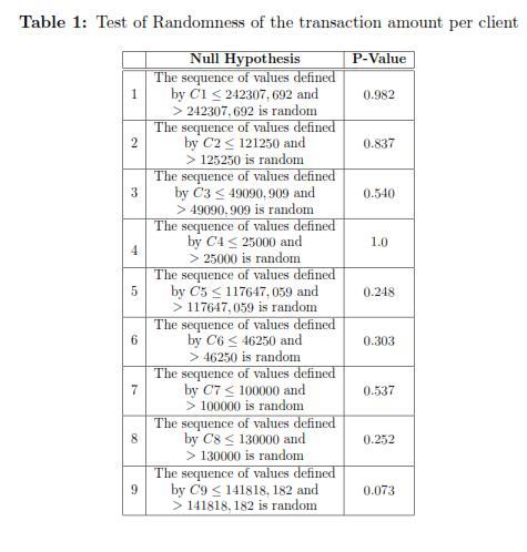
Subsequently, because the logistic model with random intercept assumes that the observations are independent, a test of runs was implemented; the results obtained are shown in Table 1. Using the mean as a measure for calculating the runs, most of the amounts of the individual transactions were categorized as independent (random). In particular, for the client 1 were obtained 8 runs.

4.3 Selection of variables

In the database there are two groups: that one where there are clients who were victims of fraud during a defined time period, and another one where there are persons who have not detected any fraudulent transactions. Using these groups, the response variable is defined as y: Marca (fraudulent transaction). Note that the observed variable is Bernoulli type. The possible independent variables in the model initially are: identification number (ID), type of ID, month, day and time when the transaction occurred, the device used for made the transaction, the channel used for the transaction (channel 1 or channel 2), the name and location of the device, the type of transaction (withdrawal, payment or transfer), the result of the transaction (successful or not ), the transaction amount (amount), type of individual (individual or business), date when individual is linked to the organization, monthly income and expenses of individuals.

Subsequently, the correlation coefficients between these variables were examined. According to the results, there is a significant correlation between the ID, type of ID and date when the individual got linked to the organization, this relation is expected because there are people of all ages who are linked to the bank after obtained their majority; it is also possible to find individuals, business or foreign persons, leading to different types of Nit.

Additionally, the month of the transaction is related to the amount of the transaction (r = 0.8, p - value < 0.05), and to the existence of fraud (r = 0.862, p - value < 0.05); this is explained by the fact that there are months in which people must make more payments than others (start year, end of year). In addition, according to information provided by the experts, there are months where fraud is most evident.

Variables as day and hour of the transaction are correlated with the rest of the variables; however the relation is not statistically significant. The relation is produced because there are certain days of the month with most probability to have transactions and obviously there are individuals who manage sums higher than average people (or vice versa).

The transaction amount is related to the existence of fraud (r = 0.82, p - value < 0:05), it is understood because there is fraud just if people withdraw money, which is equal to say that the transaction amount is greater than 0. Similarly, this variable depends on the transaction code (r = 0.9, p - value < 0:05) (which is linked directly to the device), so the existence of fraud is related to the device, although it can be due to that most of detected fraud have been made through ATMs.

The value of incoming and outgoing, are related to the amounts of the transactions (people do not spend more money than they have in their savings accounts), and the day (in some days there are more transactions). Moreover, when considering the variable Marca, there is a relationship between it and the month of the transaction. It has significant correlation with variables such as day of the transaction (r = 0.93, i - value < 0:05), hour of transaction (r = -0:96, p - value < 0:05), the transaction code and the transaction amount.

Finally, the explanatory variables, related to the absence or presence of fraud, are: channel, device code, transaction amount, month, day and time of the transaction.

However, given that fraud can be categorized using variables such as the type of device and therefore the type of transaction, they are not going to be eliminated (represented by transaction code). While variables like: Total Debts, Nit type, incoming, outgoing and document type are discarded to fit the model.

4.4 Model

The proposed model considers a random intercept per individual which represents the variability of each of them. This intercept is assumed to be a random variable distributed N(0, σ²), so estimating it, generates a fraud detection model per person due to the model is taking into account the variability of each transactions per individual. However, every estimated models have in common the coefficients associated with the rest of explanatory variables. In this model, the value of the coefficient indicates the importance of its associated variable, for this reason, the classifications of transactions will be calculated using the weight (coefficient) associated to each variable; a negative value decreases the probability of a fraud (Marca=1), while a positive value means that the probability increases [19].

It was adjusted using the GLMM package of R, with a database which contains 799 fraud detected transactions and 4854 transactions in a defined period of time. The results are shown in Table 2.

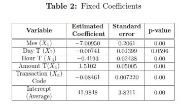
To estimate the model, some transformed variables were used to have consistency between the weights of each variable (coefficients); but according with the results, the variable related to the day when the transaction was made, is not significant, however, intuitively, this variable does not have multicolineality with others because its standard deviation is not very large; so, under supervision, this variable will be used for estimating the model. On the other hand, the month and the amount of the transaction are the variables that contribute most to the weight; however the month is the variable that most decreases the probability, while the amount increases the probability. The day and the code of the transaction have the lesser weight, so they contribute less (in a negative way.) In general terms, the model fitted to the i-th individual is

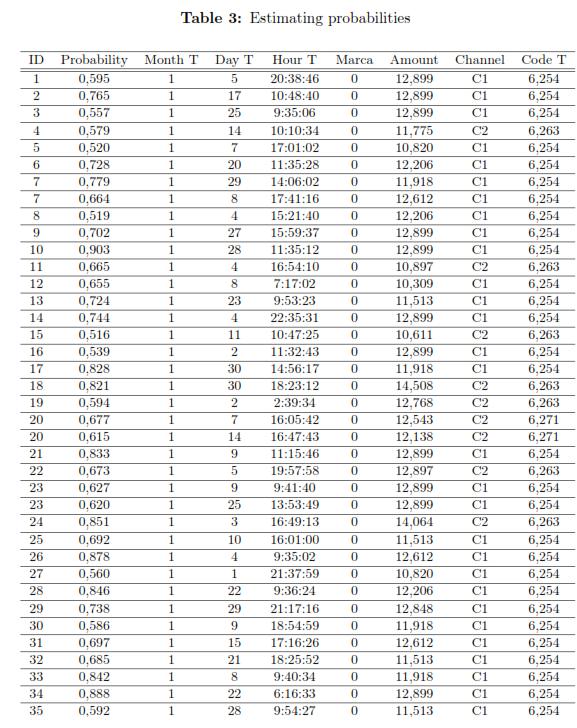
To specify the model for the individual i, the estimation of its intercept i must be considered. In the results, it is observed that for any individuals the month of the transaction, date, time and code transaction contribute negatively to the likelihood that the transaction be suspicious, but as increases the amount of the transaction , the likelihood also increases. Table 3 shows the estimated probabilities of fraud for some individuals in the database.

4.5 Model Evaluation

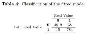
As indicated by [1], when a fraud detection model is estimated, it is necessary to take into account the sensitivity and specificity of its classification.

From the information shown in Table 4, specificity, sensitivity, bad classification rate (bcr) and good classification rate (gcr) were calculate: bcr=0.009371 gcr=0.9906 sensitivity=0.9922 specificity=0.9812 According to the literature it is preferable to have a lower misclassification rate because it indicates that the model has few mistakes, while the value of the rate of good classification (gcr) close to 1 is preferred. The sensitivity measures how good are the classifications of the model with the true positives, and specificity measures how good are the classifications of the model with the true negatives. The estimated model with random intercept has very good results, but it is clear that frauds are subject to verification.

According to tests conducted with other mixed logistic models with different combinations of variables, the model with better results in terms of gcr, bcr, sensitivity and specificity was the proposed one in this section.

4.6 Comparison with an Artificial Neural Network

In order to evaluate the performance of a mixed logistic model in comparison with the traditional techniques for detecting fraud, an Artificial Neural Network (ANN) was implemented using the variables which were utilized for estimating de mixed logistic model; also, different network architectures were applied. The ANN was selected because is the conventional method that has shown better results [see [12]].In this case it was found that the ANN did not perform as well as the mixed logistic model. The best ANN was trained using variables like Day T, Hour T and Amount T, its rates were: gcr = 0.8587, bcr = 0.1515, sensitivity= 0.8048 and specificity= 0.8959; while rates for the ANN that was trained with the same variables using in the fitted mixed logistic regression were: gcr = 0.8233, bcr = 0.1868, sensitivity= 0.7594 and specificity= 0.8714. The weak results, obtained from the ANN, can be related to the methodology used in the ANN because it estimated a general model for individuals and it was not possible to obtain a model per person as it does the logistic mixed model, that considers the different behaviours of clients.

5 Conclusions

According to the correlation analysis between variables, the found relationships coincide with the information provided by the experts. In this way, arguably that fraud is stationary, so it has to be analysed taking into account the month, the day and the hour of the transactions. Besides, type, amount and channel of the transaction should be used for fitting the model and for determining patterns for different types of fraud.

The generalized linear mixed model generates favourable results; however, it is necessary running the model for each individual as it is built with random intercepts unique per person. This, though computationally can be a disadvantage, within models is an advantage, as it would have a single representation to describe the variability of each individual. But, a high volume of historical information is required to build a profile per individual and estimate more precise models with a high quality outputs.

As future work, it is proposed estimating the model to groups of individuals more susceptible according to its characteristics (females, old people); on the other hand, it is also possible to fit a more complex model, involving variables such as type of fraud, other kind of transactions (not only financial), among others.

References

1. E. Ngai, Y. Hu, Y. Wong, Y. Chen, X. Sun, ''The application of data mining techniques in financial fraud detection: A classification framework and an academic review of literature'', Decision Support Systems, vol. 50, n.o 3, pp. 559-569, feb. 2011. [ Links ] Referenced in 222, 234

2. P. Chan, W. Fan, Andreas, A. Prodromidis, S. J. Stolfo, ''Distributed Data Mining in Credit Card Fraud Detection'', IEEE Intelligent Systems, vol. 14, n.o 6, pp. 67-74, 1999. [ Links ] Referenced in 223, 228

3. J. Dorronsoro, F. Ginel, C. Sanchez, C. Cruz, ''Neural fraud detection in credit card operations'', IEEE Transactions on Neural Networks, vol. 8, n.o 4, pp. 827 -834, jul. 1997. [ Links ] Referenced in 223, 228

4. I-C. Yeh, C. Lien, ''The comparisons of data mining techniques for the predictive accuracy of probability of default of credit card clients'', Expert Syst. Appl., vol. 36, n.o 2, pp. 2473-2480, mar. 2009. [ Links ] Referenced in 223, 228

5. T-S. C. Rong-Chang Chen, ''A new binary support vector system for increasing detection rate of credit card fraud.'', International Journal of Pattern Recognition and Artificial Intelligence (IJPRAI), vol. 20, n.o 2, pp. 227-239, 2006. [ Links ] Referenced in 223, 228

6. Abhinav Srivastava, Amlan Kundu, Shamik Sural, Arun K. Majumdar. Credit card fraud detection using hidden Markov model. IEEE Transactions on Dependable and Secure Computing, vol. 5, no1, pp. 37-48, 2008. [ Links ] Referenced in 223, 228

7. J. Quah, M. Sriganesh, ''Real-time credit card fraud detection using computational intelligence'', Expert Systems with Applications, vol. 35, n.o 4, pp. 1721- 1732, nov. 2008. [ Links ] Referenced in 223, 228

8. Vladimir Zaslavsky, Anna Strizhak, ''Credit Card Fraud Detection Using Self- Organizing Maps'', Information & Securit, vol. 18, n.o 48, pp. 48-63, 2006. [ Links ] Referenced in 223, 228

9. R. Bolton, D. Hand, ''Statistical Fraud Detection: A Review'', Statist. Sci., vol. 17, n.o 3, pp. 235-255, ago. 2002. [ Links ] Referenced in 223, 228

10. Linda Delamaire, Hussein Abdou, John Pointon, ''Credit card fraud and detection techniques: a review'', Banks and Bank Systems, vol. 4, n.o 2, pp. 57-68, 2002. [ Links ] Referenced in 223, 228

11. E. Aleskerov, B. Freisleben, y B. Rao, ''CARDWATCH: a neural network based database mining system for credit card fraud detection'', in Computational Intelligence for Financial Engineering (CIFEr), 1997., Proceedings of the IEEE/IAFE 1997, 1997, pp. 220 -226. [ Links ] Referenced in 223

12. E. Kirkos, C. Spathis, Y. Manolopoulos, ''Data Mining techniques for the detection of fraudulent financial statements'', Expert Systems with Applications, vol. 32, n.o 4, pp. 995-1003, may 2007. [ Links ] Referenced in 223, 234

13. C. Whitrow, DJ. Hand, P. Juszczak, D. Weston, ''Transaction aggregation as a strategy for credit card fraud detection'', Data Mining Knowledge Disc, vol. 18, n.o 1, pp. 30-55, 2009. [ Links ] Referenced in 223

14. D. Sánchez, M. A. Vila, L. Cerda, y J. M. Serrano, ''Association rules applied to credit card fraud detection'', Expert Systems with Applications, vol. 36, n.o 2, Part 2, pp. 3630-3640, mar. 2009. [ Links ] Referenced in 223

15. Helen Brown, Robin Prescott. Applied Mixed Models in Medicine, Statistics in Practice, 2001. [ Links ] Referenced in 225

16. ''Mixed Models: Theory and Applications''. [Online]. Available: http://www.dartmouth.edu/ [Accessed: sept-2011] [ Links ]. Referenced in 226

17. M. Quintana, A. Gallego, M. Pascual, ''Aplicación del análisis discriminante y regresión logística en el estudio de la morosidad en las entidades financieras. Comparación de resultados'', Pecunia: revista de la Facultad de Ciencias Económicas y Empresariales, vol. 1, pp. 175-199, 2005. [ Links ] Referenced in 227

18. A. Alderete, ''Fundamentos del Análisis de Regresión Logística en la Investigación Psicológica'', Revista Evaluar, vol. 6, pp. 52-67, 2006. [ Links ] Referenced in 227

19. Brady West, Kathlen Welch, Andrzej Galecki. Linear Mixed Models: A practical guide to using statistical software, Chapman & Hall,2007. [ Links ] Referenced in 231