


Serviços Personalizados
Journal
Artigo
 Inglês (pdf)
 Artigo em XML
 Referências do artigo
 Enviar este artigo por email
Indicadores
-
 Citado por SciELO
 -
 Acessos
Links relacionados
-
 Citado por Google
 -
 Similares em
SciELO
Similares em
SciELO -
 Similares em Google
Compartilhar

 Permalink
Ingeniería y Ciencia
versão impressa ISSN 1794-9165
ing.cienc. vol.9 no.17 Medellín jan./jun. 2013
ARTÍCULO ORIGINAL
Two-Dimensional Meshless Solution of the Non-Linear Convection-Diffusion-Reaction Equation by the Local Hermitian Interpolation Method
Solución bidimensional sin malla de la ecuación no lineal de convección-difusión-reacción mediante el método de Interpolación Local Hermítica
Carlos A. Bustamante Chaverra1, Henry Power2 , Whady F. Florez Escobar3 and Alan F. Hill Betancourt4
1 MSc. in Energetic Systems, carlos.bustamante@upb.edu.co, Universidad Pontificia Bolivariana, Medellín, Colombia.
2 PhD. in Computational Mechanics, henry.power@nottingham.ac.uk, University of Nottingham, Nottingham, UK.
3 PhD. in Computational Mechanics, whady.florez@upb.edu.co, Universidad Pontifica Bolivariana, Medellín, Colombia
4 MSc. in Technology Management, Universidad Pontifica Bolivariana, Medellín, Colombia.
Received: 18-04-2012, Acepted: 01-02-2013 Available online: 22-03-2013
MSC: 65H20, 65N35
Abstract
A meshless numerical scheme is developed for solving a generic version of the non-linear convection-diffusion-reaction equation in two-dimensional domains. The Local Hermitian Interpolation (LHI) method is employed for the spatial discretization and several strategies are implemented for the solution of the resulting non-linear equation system, among them the Picard iteration, the Newton Raphson method and a truncated version of the Homotopy Analysis Method (HAM). The LHI method is a local collocation strategy in which Radial Basis Functions (RBFs) are employed to build the interpolation function. Unlike the original Kansa's Method, the LHI is applied locally and the boundary and governing equation differential operators are used to obtain the interpolation function, giving a symmetric and non-singular collocation matrix. Analytical and Numerical Jacobian matrices are tested for the Newton-Raphson method and the derivatives of the governing equation with respect to the homotopy parameter are obtained analytically. The numerical scheme is verified by comparing the obtained results to the one-dimensional Burgers' and two-dimensional Richards' analytical solutions. The same results are obtained for all the non-linear solvers tested, but better convergence rates are attained with the Newton Raphson method in a double iteration scheme.
Key words: Radial Basis Functions, Meshless methods, Symmetric method, Newton Raphson, Homotopy Analysis Method.
Highlights
• Non-linear convection-diffusion equation is solved accurately by a meshless method. • 1D Burgers' and 2D Richards' equations are solved by using several nonlinear solvers. • The best convergence rate is achieved when employing the Newton-Raphson method.
Resumen
Un método sin malla es desarrollado para solucionar una versión genérica de la ecuación no lineal de convección-difusión-reacción en dominios bidimensionales. El método de Interpolación Local Hermítica (LHI) es empleado para la discretización espacial, y diferentes estrategias son implementadas para solucionar el sistema de ecuaciones no lineales resultante, entre estas iteración de Picard, método de Newton-Raphson y el Método de Homotopía truncado (HAM). En el método LHI las Funciones de Base Radial (RBFs) son empleadas para construir una función de interpolación. A diferencia del Método de Kansa, el LHI es aplicado localmente y los operadores diferenciales de las condiciones de frontera y la ecuación gobernante son utilizados para construir la función de interpolación, obteniéndose una matriz de colocación simétrica. El método de Newton-Rapshon se implementa con matriz Jacobiana analítica y numérica, y las derivadas de la ecuación gobernante con respecto al paramétro de homotopía son obtenidas analíticamente. El esquema numérico es verificado mediante la comparación de resultados con las soluciones analíticas de las ecuaciones de Burgers en una dimensión y Richards en dos dimensiones. Similares resultados son obtenidos para todos los solucionadores que se probaron, pero mejores ratas de convergencia son logradas con el método de Newton-Raphson en doble iteración.
Palabras clave: Funciones de Base Radial, Métodos sin malla, Método Simétrico, Newton-Raphson, Método de Homotopía.
1 Introduction
The Radial Basis Functions (RBFs) have been widely used in global and continuous interpolation of scattered data sets. Moreover, RBF collocation by using Multiquadric (MQ), Thin Plate Spline (TPS) and Inverse Multiquadric (IMQ) functions was considered as one of the best numerical techniques for multidimensional interpolation, in terms of accuracy and ease of implementation, among several schemes tested by Franke [1]. It is fair to mention, that the TPS functions are optimal 2 interpolants since they minimizes the functional ∫Rn 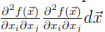 for i = 1,
  , n and j = 1, , n. Recently, the RBFs have been employed as the base of meshless collocation approaches for solving partial differential equations (PDEs). The use of RBF interpolation technique has become the foundation of the RBF meshless collocation methods for the solution of PDEs, since the pioneer work on the Unsymmetric method by Kansa [2]. Kansa use the MQ function to obtain an accurate meshless solution to the advection-diffusion and Poisson equations without employing any special treatment for the advection term (upwinding), due to the high order of the resultant scheme and the intrinsic relationship between governing equations and the interpolation. This strategy involved all the scattered nodes that cover the domain and therefore it produced a global fully populated matrix. With the aim of improving the Kansa's Method, Fasshauser [3] use Hermite interpolation to construct an RBF interpolating function which gives a non-singular symmetric collocation matrix. He concludes that the Hermitian (Symmetric) method performs slightly better than the Kansa (Unsymmetric) method. Jumarhon et al. [4] obtain a similar improvement using the Symmetric method and more recently Power and Barraco [5] attain better results by employing the Symmetric method for a variety of problems including convection diffusion equation. Later, La Rocca et al. [6] implement the Symmetric method in the context of the Method of Fundamental Solutions (MFS) to solve transient convection- diffusion problems showing better accuracy of the scheme in the cases of strong variable velocity field with respect to the traditional formulation. Also, Chinchapatnam et al. [7] solve the convection-diffusion equation using several RBFs by Symmetric and Unsymmetric method. Their results are in agreement with those presented by Fasshauser [3].
Full-domain RBF methods exhibit high-order convergence rates of the L2-norm of the difference between the interpolation function and a test (analytical) function in terms of the upper bound of the distances between points (see [8] for the MQ case), and are used by many authors to solve variety of problems (Laplace, Poisson, Helmholtz and Parabolic equations) showing better accuracy compared to traditional methods [9], [10],[11],[12]. Nevertheless, the fully-populated matrix systems they produce lead to poor numerical conditioning as the size of the data-set increases. This problem is described by Shaback [13] as the uncertainty relation; better conditioning is associated with worse accuracy, and worse conditioning is associated with improved accuracy. As the system size is increased, this problem becomes more pronounced. Many techniques have been developed to reduce the effect of the uncertainty relation, such as RBF-specific preconditioners [14] and adaptive selection of data centres [15]. However, at present the only reliable method of controlling numerical ill-conditioning and computational cost as problem size increases is through domain decomposition (see, for example, [16],[17],[18],[19]).
One of the first attempts in this direction is made by Lee et al. [20] who propose the local MQ approximation in which only the nodes inside the influence subdomain of one central node are used in the Unsymmetric method for solving the Poisson equation. Based on the above development Sarler and Vertnik [17] create an explicit scheme to solve transient diffusion equation. Later on, other schemes are implemented by modifying traditional methods using Symmetric and Unsymmetric method. Wright and Fornberg [19] generalise the Finite Difference Method (FDM) using RBF Hermite interpolation attaining high order local approximations. Moroney and Turner [21],[22] apply the RBF interpolation in the Finite Volume Method (FVM) to reconstruct gradients in a two- and three-dimensional non-linear diffusion problems by the Unsymmetric method. More recently, Orsini et al. [23] solve the diffusion convection equation by using the FVM and the Hermitian (Symmetric) and the Unsymmetric interpolation schemes. In the pure meshless RBF collocation strategies there are also recent developments. Divo and Kassab [18] solve the non-isothermal flow problem by implementing a localized Radial Basis method based on the formulation proposed in [17] and using a sequential algorithm. Afterwards, Stevens et al. [24] implement the Local Hermitian Interpolation Method (LHI) to solve transient and non-linear diffusion problems. Unlike the method proposed in [18], Stevens et al. [24] employ the Symmetric method considering the boundary operator at the local level. Stevens et al. [25] solve accurately the two and three dimensional convection diffusion equation by LHI method including the PDE operator and PDE centres in the approximation of the solution field for each local domain. The LHI method is the scheme used in the present work focusing in the solution of a generic version of the non-linear convection diffusion reaction equation.
Newton like methods have been widely use in the solution of non- linear system of equations [26],[27]. However, in the case of non-linear systems which arise from the discretization of non-linear PDEs other strategies are often used regarding a straightforward implementation as the Picard iteration scheme. For instance, Cui and Yue [28] develop a FDM scheme for systems of non-linear parabolic and hyperbolic differential equations by employing a Picard iteration strategy and Mohan et al. [29] employ Picard iteration in the solution of a non-linear diffusive transport equation. Despite of the ease of implementation, the Picard iteration strategy is limited by its slow convergence in terms of the L2-norm of the difference between the function value at present and previous iteration and its inability of dealing with strong non- linearities unless variable transformations are available (for example see [30]). Nevertheless, such transformations require non-trivial operations in terms of computational cost and cannot be applied for general forms of the non-linear terms, i.e. each type of non-linear term needs a specific transformation to weaken its influence on the problem.
The Homotopy or continuation methods for the solution of non- linear equation systems have been developed with the aim of reducing the influence of the initial guess in the validity of the approximation [31]. For solving non-linear PDEs, Liao [32] proposes the Homotopy Analysis Method (HAM) with the aim of generalising the Boundary Element Method (BEM), obtaining accurate solutions for several linear and non-linear problems. Also, Liao [33] solves transient non-linear heat transfer in two-dimensional domains by using a fully implicit FDM for time discretization and the BEM for the spatial discretization in the sense of the HAM formulation. The numerical results obtained by Liao for a third order formulation are enough accurate in comparison to those given by an iterative BEM scheme showing that HAM is an efficient technique compared to Picard iterative schemes. Later on, the HAM in conjunction to numerical methods for the PDE spatial discretization has been applied to obtained numerical solution for a variety of non-linear problems (see [34],[35],[36]).
In this paper a meshless numerical scheme is proposed to solve a two- dimensional generic convection-diffusion-reaction equation by employing the LHI method in conjunction to several strategies to solve the resulting set of non-linear equations. Among them the Picard iteration scheme, Newton Raphson method and a truncated version of the Homotopy Analysis Method. The main goal of this work is to evaluate which of the mentioned non-linear solvers performs better, in terms of computational efficiency, when solving the non-linear convection-diffusion-reaction equation discretized by the LHI method. In the following section the LHI solution of the generic convection-diffusion-reaction equation is detailed and the resulting non-linear equation system is presented. Then the application of the non-linear solvers to the resulting LHI discretization equation is explained starting with the Picard Iteration and following with the Newton Raphson method and the HAM. Afterwards the numerical results for the one-dimensional Burgers' equation and two- dimensional Richards' equation are obtained and the convergence rates of the different solvers are compared.
2 The Local Hermitian Interpolation Method
The RBFs are characterised for its only dependence on the Euclidian distance between test and trial points and its radial symmetric, i.e. its value does not change when the coordinates system is rotated. Other important features are the monotonically increasing and decreasing of the function with the distance from the origin (test point), adjustable softness and excellent convergence properties. The RBFs more often used in interpolation are presented in the Table 1. Where r =  x - ξj is the Euclidian distance between a domain node x and a trial point ξj.
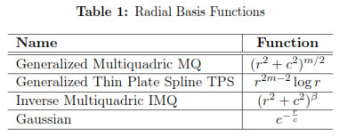
The MQ function converges exponentially and, like TPS, is conditionally positive define of order m > 0, since it is necessary to add a polynomial term of order m - 1 to guarantee a non-singular resulting matrix. Besides, MQ has a shape parameter c which allows to change the function slope near the collocation point. For small values of c the function turns in a cone shape, that will flattens as the shape parameter increases. The TPS behaves well in the interpolation of multivariable functions and does not have adjustable parameter, although it converges linearly. The Gaussian and IMQ functions (β < 0) are positive define and hence requires the addition of a polynomial term. In the present work the MQ function is used considering its exponentially convergence.
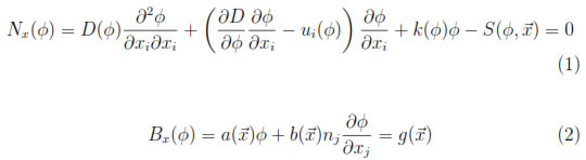
A generic non-linear diffusion-convection-reaction problem is given by the governing PDE (1) and the boundary condition (2). The functions D, and k are, respectively, the diffusive, convective and reactive coefficients and S is the source term. The coefficients a and b are functions of the position and according to its values a specific boundary condition is applied at each boundary point. The outward normal vector is denoted as
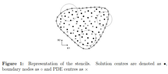
To implement the LHI method it is necessary to cover the solution domain with two sets of scattered points as shown in Figure 1. The two sets of points are the nodes where the solution and the PDE will be enforced by interpolation; hence they are called, respectively, solution nodes and PDE centres. Each solution node has an associated stencil, which is the subdomain where a specific interpolation function is valid. The stencil (big circles in Figure 1) contains three kinds of points which are the solution nodes, the PDE centres and the boundary points when the stencil intersects the domain boundary. For more information about the effect of the stencil nodal distribution on the performance of the method, see [24],[25].
In the LHI method, the dependent variable is locally approximated by a function in terms of RBFs. The Hermitian characteristic of the method is a consequence of using the governing PDE and the boundary operators to define the local approximation. For solving linear problems the governing PDE operator can be used directly, while in the non-linear case some linearized version of the operator has to be applied. In the present work, an auxiliary linear operator Lx is built by using known values of the dependent variable Φ* to compute the equation coefficients as shown in the following expression:

Then, the dependent variable Φ can be approximated by the expression
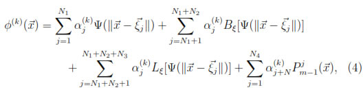
where k refers to the stencil number, Ψ is the RBF and N1, N2 and N3 are, respectively, the number of solution centres, the boundary points and the PDE centres contained in the stencil k. N4 refers to the number of polynomial terms which depends on the dimensions of the problem and the RBFs used.
Like in the Symmetric method [3],[25], the collocation procedure is performed by evaluating the variable approximation (4) at the solution nodes, the approximated boundary condition Bx (Φ(k)( )) at the boundary points and the governing PDE Lx(Φ(k)()) at the PDE centres. Considering the generic operator Ξ[] the collocation procedure can be expressed as:
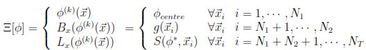
with Φcentre as the unknown variable value, g() as the known function of the boundary condition, S(Φ*,) equivalent to the known source term function and NT = N1 + N2 + N3. Then a linear equation system A(k)αk = d(k) is obtained where the symmetric matrix A(k) and the column vector d(k) are defined as:
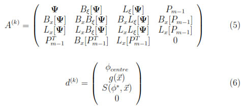
The matrix A(k) is non-singular as long as Ψ is chosen appropriately, i.e. MQ, TPS, IMQ functions [6], and provided that no two data-centres sharing linearly dependent operators are placed at the same location [25]. According to the equations (5) and (6), the variable Φ at a point located inside the stencil k is given by the equation (7),

with

So far a local interpolation equation is obtained for the stencil k, considering the coefficient α(k) in terms of the variable values at the solution centres included in the stencil. Then the original operator of the problem Nx is applied to the dependent variable expressed as (7) and the resulting equation is evaluated at the central solution point k, to obtain the non-linear expression (9) which relates the unknown variable values contained inside the stencil k.

By applying the equation (9) to each one of the N stencils related to the N solution centres scattered throughout the domain, a set of N non- linear equations is obtained. It is important to notice that the solution attained after solving the non-linear system is not the final solution since the local interpolation is performed by using the values of the dependent variable at the last iteration. Hence a double iteration algorithm is required to achieve the final solution, i.e. an outer loop where the coefficients in the interpolation matrices, which are functions of Φ and are contained in the PDE operator L[.], are updated, and an inner loop where the non-linear system of equations (9) is solved. The solution of the non-linear equation system, the double iteration algorithm and the possibility of solving the problem without the mentioned outer iteration are discussed in the next section. For a deeper analysis of the Hermitian collocation method as a spatial discretization strategy, see [4],[24],[25] where the order of convergence of the L2-norm of the error as a function of the nodal distance is studied as well as the computational complexity of the algorithm implemented, and [5],[24] where problems with non-homogeneous Neumann boundary conditions are solved and the problem of instability in the solution is addressed.
3 Solution of the non-linear convection-diffusion-reaction equation
Four strategies for solving the non-linear equation system which arises from the LHI discretization of the generic non-linear convection diffusion reaction equation (1) are tested. The strategies are the Picard Iteration, Newton Raphson method with double iteration, Newton Raphson method with single iteration and the truncated Homotopy Analysis method with double iteration.
The Picard iteration is the simplest strategy used here to solve the non-linear system. In this case, the linear problem represented by equation (3) is solved iteratively until convergence. It is important to mention that the equation (3) is equivalent to the expression (1) after substituting the coefficient and source term values with the ones obtained in the previous iteration. The solution of the linear problem is performed as it is shown by Steven et al. [24]. The stop criterion is the magnitude of the difference between the solution at the last and the current iteration 
 +1 -.
+1 -.
3.1 Newton-Raphson method
Newton-like methods has been widely used for solving non-linear equation systems. In this case, the Newton-Raphson method is employed with the aim of increasing the convergence rate and decreasing the computing times respect to the Picard iteration proposed above. The Newton Raphson method is a good option since it shows quadratic convergence rate when the initial guess is close to the problem solution [26] as long as the solution function is smooth. In this sense, the use of MQ functions for the approximation is appropriate since they are infinitely differentiable [1]. For equation systems, the solution of the problem is given by the following equation:

where [J] is the Jacobian matrix, [Φ] is a column vector containing the solution at the iteration indicated by the super index and [F (Φn-1)] is a column vector with the non-linear functions evaluated at the last iteration. In this case, the non-linear functions are the resulting equations of the LHI spatial discretization and are given by the expression (9).
Both numerical and analytical Jacobian matrices are computed with the aim of verifying the performance of the scheme using the numerical one. The numerical Jacobian is obtained by means of a finite difference strategy according to the equation (11), where ΔΦ is a small perturbation applied to the Φj variable. The perturbation ΔΦ is found experimentally for each problem, i.e. several values are used and the greatest one with which the algorithm converges to an accurate solution is selected.

The analytical Jacobian Jaij is obtained by differentiating with respect to the variable Φj the non-linear function fi, which is the expression (9) applied to the stencil i. Regarding the interpolation matrix [A](k) are not in terms of Φj but  , the analytical Jacobian Jaij is given by the expression

where the Einstein summation convention is considered except for the terms with the index in parenthesis. The derivatives of Φ(i), its gradient and its Laplacian with respect to the variable Φj can be expressed as equations (13),(14) and (15) according to (7).

Two algorithms have been implemented to solve the non-linear problem by the Newton-Raphson method. The first of them is the single iteration scheme in which the numerical Jacobian is computed with the interpolation matrix [A] as a function of the solution Φ, i.e. no linearization of the differential operators employed in the interpolation is required. The single iteration algorithm can be described as follows.
1. Enter the initial guess Φ0.
2. Evaluate the non-linear equation (9) including the interpolation coefficients [α] in terms of Φ0
3. Find the numerical Jacobian according to the expression (11) by evaluating the non-linear set of function (9) in Φj +ΔΦ with j being the index of the solution nodes in the stencil. The interpolation coefficients are calculated for each component of the Jacobian and, in consequence, each local equation system has to be solved as many times as the number of solution nodes included in the stencil.
4. Compute the new value of the solution Φn+1 by using the equation (10).
5. Check the tolerance criterion +1 - < tol. End, if it is satisfied, or go to the step 2 with Φ0 = Φn+1, otherwise.
The second algorithm implemented requires a double iteration or two loop strategy since the non-linear problem is solved with constant interpolation coefficients [α]. Thus the problem is split in a local linear problem that is solved in an external loop and a global non-linear problem which is solved by the Newton-Raphson method in an internal loop. The algorithm is given by the following sequence.
1. Enter the initial guess Φ0.
2. External loop: Compute the interpolation coefficients for each stencil by evaluating the interpolation matrix [A] at the current solution value Φn (or Φ0 at the first iteration)
3. Internal loop: Evaluate the non-linear equation (9) in terms of Φn to obtain [F (Φn)] and calculate the numerical or the analytical Jacobian according to the expressions (11) or (12), respectively.
4. Compute the new value of the solution Φn+1 by using the equation (10).
5. Check the tolerance criterion for the non-linear or internal loop +1 - < tolnl. Go to step 6, if it is satisfied, go to step 3 with Φn = Φn+1, otherwise.
6. Check the tolerance criterion for the linear or external loop +1 -  < tol. If it is satisfied, Φn+1 is the final solution, otherwise go to step 2 with Φ0 = Φn+1.
3.2 Truncated Homotopy Analysis Method
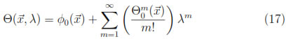
The Homotopy Analysis Method (HAM) proposed by Liao [32] as a generalisation of the BEM is employed here for the solution of the non- linear convection diffusion reaction problem. The HAM solves the non- linear problem as a combination of linear auxiliary solutions. The non- linear solution is expressed as the homotopy Θ which is constructed by performing a continuous deformation of the initial linear solution Φ0. The zeroth order deformation equation is given by expression (16), where Lx and Nx refer, respectively, to the linear and the non-linear differential operators as they are defined in the linearized equation (3) and the governing PDE (1). The homotopy Θ is a function of the domain and the parameter p  [0, 1] and, according to the deformation equation, Θ(, 0) = Φ0 and Θ(, 1) = Φ.

The homotopy function Θ is considered smooth enough to assure the continuity of its derivatives respect to the parameter p. Then it is possible to define Θ as a expansion in Taylor series according to the expression (17), where 0 < λ < ρ < 1 with λ being a necessary parameter when the convergence ratio ρ is less than the unit. For brevity the m-order derivative of Θ respect to p for p = 0 is written as  ().
().
The iterative formulation given by the following equation is obtained from (17) when the series is truncated at m = M, being M the order of the formulation.
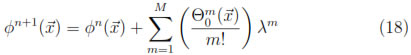
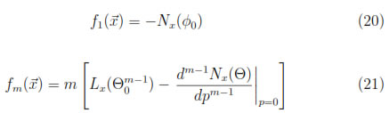
Hence, the iterative solution of the non-linear problem is achieved by computing the mth-order derivatives of the homotopy (m = 1, . . . , M). Thus differentiating the zeroth order deformation equation (16) with respect to the parameter p, an expression for the m-th order homotopy derivative is obtained. The generalised mth-order deformation equation can be expressed as
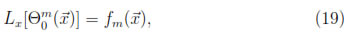
with the function fm given by equation (20) when m = 1 and (21) when m > 1.
The equation (19) is solved for as a boundary value problem with the following boundary condition obtained from the original condition (2) as in the formulation proposed by Liao [33].

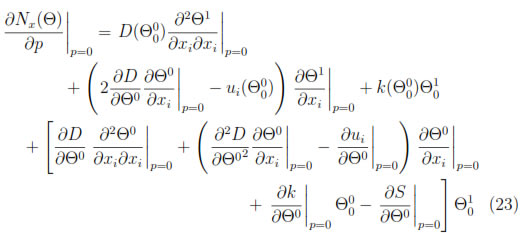
In this work, the homotopy series is truncated at M = 2. Hence, just the first derivative  has to be calculated. The equation (23) results from differentiating the generic expression (1) with respect to p and evaluating it at p = 0. After solving the first order deformation equation for
  , the equation (23) is evaluated by reconstructing the
 and gradients and Laplacians at the stencil centre using the LHI discretization.
To implement the HAM, a double iteration algorithm is used with the aim of updating both the local interpolation operators and the auxiliary linear operator Lx. The HAM solution is achieved by performing the following algorithm.
1. Enter the initial guess Φ0.
2. External loop: Compute the interpolation coefficients for each stencil by evaluating the interpolation matrix [A] at the current solution value Φn (or Φ0 at the first iteration).
3. Internal loop: Sequentially, calculate the right hand side of the mth-order deformation equation (19) and solve the resulting linear boundary value problem for each m, with m = 1, . . . , M.
4. Compute the new value of the solution Φn+1 by using the equation (18).
5. Check the tolerance criterion for the non-linear or internal loop +1- < tolnl. Go to step 6, if it is satisfied, go to step 3 with Φn = Φn+1, otherwise.
6. Check the tolerance criterion for the linear or external loop +1 - < tol. If it is satisfied, Φn+1 is the final solution, otherwise go to step 2 with Φ0 = Φn+1.
4 Numerical results
The non-linear LHI scheme with the algorithms presented in the last section is verified by solving one and two-dimensional problems involving non-linear PDEs. The four non-linear solvers are the Newton Raphson method with single iteration and numerical Jacobian (NR1INJ), the Newton Raphson method with double iteration and analytical Jacobian (NR2IAJ), the Newton Raphson method with double iteration and numerical Jacobian (NR2INJ) and the Homotopy Analysis method with M = 2 (HAM2). All cases are solved in a PC INTEL CORE 2 DUO, 2.66 GHz, 2 GB RAM, using a FORTRAN 90 code with the IMSL libraries for linear algebra calculations.
The first problem is the one-dimensional steady Burgers' equation which can be obtained from the generic form (1). In the second case, the diffusive coefficient is an exponential function of the dependent variable obtaining a non-linear PDE which represent the two dimensional steady Richards' equation. In all problems, the shape parameter value is a function c = dh, where the average distance between the central point and the rest of the points in a stencil is given by h and d is a factor specified for each problem solved.
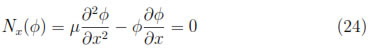
The one-dimensional steady Burgers' equation (24) is obtained by setting D = μ, u1 = Φ, k = 0 and S = 0 in the generic non-linear convection diffusion reaction equation (1).
The analytical solution of the Burgers equation with Dirichlet boundary conditions Φ(0) = u0 and Φ(L) = 0 is reported in [37] as the expression
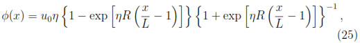
where the parameter R =  is analogous to the Reynolds number and η is the root of the non-linear algebraic expression
  = exp(-ηR), which is obtained by an independent non-linear scalar equation solver.
4.1 One-dimensional Burgers' equation
The one-dimensional solution is obtained by means of the developed twodimensional code by setting Neumann boundary conditions  i = 0 on the extreme x2-constant lines (x2 = 0.0 and x2 = 0.2). Numerical solutions for different values of the parameter R are presented in Table 2 and Figure 2.
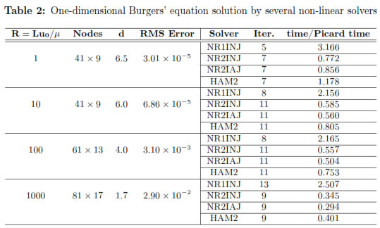
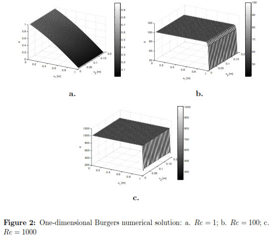
According to the numerical solutions presented in the Figure 2 it is clear that as the R value is increased the Φ-gradient near to x1 = 1.0 is higher and, in consequence, obtaining adequate numerical solutions for high R depends on the spatial accuracy of the discretization scheme. In the Table 2, the global iterations and the ratio between the CPU time spending of the employed nonlinear solver and the Picard iteration scheme are shown.
A homogeneous nodal distributions are employed and the shape parameter factor d is set experimentally. The boundary conditions are applied in the local approximation i.e. no global equation is evaluated at the boundary points. The RMS error is computed by the following equation:
where Φnum and Φ are the numerical and the analytical solution, respectively, and N the total number of nodes.
The assessment of the non-linear solvers is based on the number of global iterations and the CPU time knowing the RMS error is the same for all the computations since they are obtained by means of the same LHI spatial discretization. Therefore the same solution is attained by all the solvers tested as can be seen in Figure 3 a. for Re = 100 and Figure 4 a. for Re = 1000, in which the absolute errors on the line x2 = 0.1 are presented.
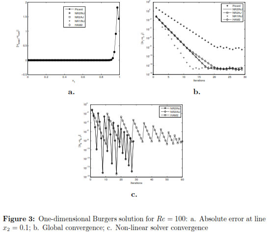
The NR1INJ strategy is the most expensive in time (2.50 to 3.16 times of the CPU time spending using Picard iteration) despite showing the highest global convergence rate and, in consequence, the fewest number of global iterations for R ≤ 100. For Re = 1000 the number of global iteration in the NR1INJ strategy is the highest due to the ill-conditioning of the local interpolation matrices which causes an inaccurate response to the small perturbations needed to compute the numerical Jacobian matrix. The double iteration strategies perform better than the single iteration one considering the CPU time spending and the stability of the method as the parameter R is increased. As shown in Figures (3) b. and (4) b. the convergence rate of the double iteration strategies are almost the same while in the NR1INJ case the rate is higher for R = 100 and smaller for R = 1000. As is expected, the Picard iteration strategy gives the lowest convergence rate.
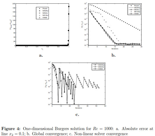
In Figures (3) c. and (4) c. the L2-norm of the absolute error between solutions at k and k-1 iterations of the internal loop are shown for the double iteration strategies. The Newton Raphson strategies (NR2INJ and NR2IAJ) present a high convergence rate similar in trend to the quadratic convergence rate expected from Newton like methods [26]. Besides, the behaviour is the same for both the analytical and numerical Jacobian cases showing that the Jacobian obtained by finite difference scheme is a suitable strategy to solve non-linear problems without the need of computing an analytical expression for the Jacobian. The HAM2 strategy requires more iterations and CPU time than the double iteration Newton Raphson schemes. The convergence rate of the HAM2 can be improved by taking a higher value of M, nevertheless the CPU time will be higher.
4.2 Two-dimensional Richards' equation
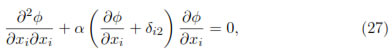
The two-dimensional Richards' equation for the steady state is obtained from the general form (1) by setting D = eαΦ, u1 = 0, u2 = -αeαΦ, k = 0 and S = 0. By doing some algebra, the Richards' equation is reduced to the expression
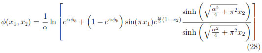
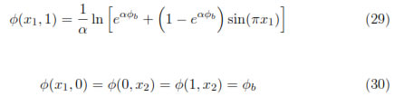
which is solved by the non-linear LHI strategies implemented. As the parameter α increases, the non-linearity becomes stronger and the gradients near to the boundaries higher, as in shown in the numerical results obtained for different α values (Figure 5). The two-dimensional domain is the square (0 ≤ x1 ≤ 1, 0 ≤ x2 ≤ 1) and the analytical solution is given by equation (28) applying the Dirichlet boundary conditions (29) and (30) [38].

The results presented in Table 3 are obtained using a homogeneous nodal distribution. The RMS error is the same for all the solvers employed and the shape parameter factor d is found experimentally as in the Burgers' equation case. The boundary conditions are applied at the local level. The number of global iterations and the CPU time increase with the parameter α but, unlike in the solution of Burgers' equation, the RMS error are much higher and it is not possible to attained a solution by using some solvers for α = 3 and α = 4.
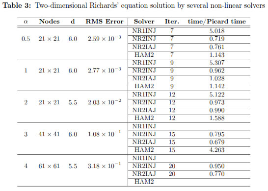
When α = 3 the NR1INJ strategy is unable to solve the problem whatever the initial values are and the HAM2 spends approximately 4 times the CPU time required by the Picard iteration strategy. In case of NR1INJ, the ill-conditioning of the interpolation matrices causes poor accuracy in the numerical Jacobian computation. The equivalence among the attained solutions is verified in the Figure 6 a. which shows the absolute error at line x2 = 0.5 for α = 3. The Figure 6 b. allows to have a qualitatively idea of the high global convergence rates which the double iteration strategies present with respect to the Picard iterative scheme. The Figure 6 c. shows the slow convergence rate of the HAM strategy in the solution of the non-linear equation system while the double iteration Newton Raphson schemes present a similar convergence rate such as in the solution of the Burgers' equation (Figure 3 c and 4 c). A small difference can be noticed between the NR2INJ and NR2IAJ being the last (analytical Jacobian) better in terms of number of iterations and CPU time. However the analytical Jacobian computation increases the input data (coefficients plus their derivatives with respect to the dependent variable) making difficult the code implementation for the solution of a generic-convection-diffusion reaction equation compared to the numerical Jacobian strategy. Finally, in the case of α = 4 the HAM2 solver fails to obtained a solution and the Newton Raphson results are attained spending less CPU time compared to the Picard iteration case.

After solving the one-dimensional Burgers' and the two-dimensional Ri-chards' equations the better non-linear equation solver to be used in conjunction to the LHI discretization is the double iteration Newton Raphson schemes NR2INJ and NR2IAJ. Although the NR2IAJ performs better than the NR2INJ, the implementation of the numerical Jacobian strategy (NR2INJ) is straightforward compared to the NR2IAJ since no analytical effort is required to compute the Jacobian. Hence the numerical results obtained above prove that the finite difference is a suitable scheme to compute the Jacobian.
5 Conclusions
A meshless procedure for the solution of the generic two-dimensional convection-diffusion-reaction equation is implemented. Several non-linear solvers for the solution of the equation system arising from the LHI spatial discretization are tested. The one-dimensional Burgers' and the two dimensional Richards' equations are solved to assess the developed non-linear solvers. Based on the number of global iterations and the CPU time, the best strategies are the Newton Raphson method in a double iteration scheme with numerical (NR2INJ) and analytical (NR2IAJ) Jacobians. The single iteration Newton Raphson (NR1INJ) scheme is more sensitive to the ill-conditioning of the local interpolation matrices and in consequence fails when the nonlinearity becomes strong. The convergence rate of the truncated Homotopy Analysis Method (HAM) with M = 2 depends on the strength of the nonlinearity, making the method unsuitable for strongly non-linear problems. The NR2INJ requires more CPU time than the NR2IAJ but its implementation for the solution of non-linear PDE systems is simpler. Therefore from the non-linear solvers tested the NR2INJ scheme is the most appropriate for the solution of generic convection diffusion reaction problems.
Acknowledgment
The present work is supported by COLCIENCIAS and Empresas Públicas de Medellín (EPM) as part of the funding provided to the project Energetic assessment of the San Fernando plant bio-solids which has been developed by the union of local academic institutions and the public utility company EPM, known as the Energy Research and Innovation Centre (CIIEN).
References
[1] R. Franke, ''Scattered data interpolation: tests of some methods,'' Math. Comp., vol. 38, pp. 181-200, 1982. [ Links ] 23, 32
[2] E. J. Kansa, ''Multiquadrics -a scattered data approximation scheme with applications to computational fluid dynamics-II solution to parabolic, hyperbolic and elliptic partial differential equations,'' Comput. Math. Appl., vol. 19, no. 8-9, pp. 127-145, 1990. [ Links ] 23
[3] F. E. Fasshauer, ''Solving partial differential equations by collocation with radial basis functions,'' Surf. Fit. Multires. Methods, pp. 131-138, 1997. [ Links ] 23, 24, 29
[4] B. Jumarhon, S. Amini, and K. Chen, ''The Hermite collocation method using radial basis functions,'' Eng. Anal. Boundary Elem., vol. 24, no. 7-8, pp. 607-611, 2000. [ Links ] 23, 31
[5] H. Power and V. Barraco, ''A comparison analysis between unsymmetric and symmetric radial basis function collocation methods for the numerical solution of partial differential equations,'' Comput. Math. Appl., vol. 43, no. 3-5, pp. 551-583, 2002. [ Links ] 23, 31
[6] A. LaRocca, A. Hernandez, and H. Power, ''Radial basis functions Hermite collocation approach for the solution of time dependent convenction-diffusion problems,'' Eng. Anal. Boundary Elem., vol. 29, no. 4, pp. 359-370, 2005. [ Links ] 24, 30
[7] P. P. Chinchapatnam, K. Djidjeli, and P. B. Nair, ''Unsymmetric and symmetric meshless schemes for the unsteady convection?diffusion equation,'' Comput. Meth. Appl. Mech. Eng., vol. 195, no. 19-22, pp. 2432-2453, 2006. [ Links ] 24
[8] W. R. Madych and S. A. Nelson, ''Multivariate Interpolation and Conditionally Positive Definite Functions,'' Math. Comput., vol. 54, no. 1, pp. 211-230, 1990. [ Links ] 24
[9] M. Zerroukat, H. Power, and C. S. Chen, ''A numerical method for heat transfer problems using collocation and radial basis functions,'' Int. J. Numer. Methods Eng., vol. 42, no. 7, pp. 1263-1278, 1998. [ Links ] 24
[10] J. Li, A. H. D. Cheng, and C. S. Chen, ''A comparison of efficiency and error convergence of multiquadric collocation method and finite element method,'' Eng. Anal. Boundary Elem., vol. 27, no. 3, pp. 251-257, 2003. [ Links ] 24
[11] A. H.-D. Cheng and J. J. S. P. Cabral, ''Direct solution of ill-posed boundary value problems by radial basis function collocation method,'' Int. J. Numer. Methods Eng., vol. 64, no. 1, pp. 45-64, 2005. [ Links ] 24
[12] S. Chantasiriwan, ''Cartesian grid methods using radial basis functions for solving Poisson, Helmholtz, and diffusion?convection equations,'' Eng. Anal. Boundary Elem., vol. 28, no. 12, pp. 1417-1425, 2004. [ Links ] 24
[13] R. Schaback, ''Multivariate interpolation and approximation by translates of basis functions,'' Approx. Theory, vol. 8, pp. 1-8, 1995. [ Links ] 24
[14] D. Brown, ''On approximate cardinal preconditioning methods for solving PDEs with radial basis functions,'' Eng. Anal. Boundary Elem., vol. 29, pp. 343-353, 2005. [ Links ] 24
[15] L. Ling and R. Schaback, ''On adaptive unsymmetric meshless collocation,'' Proceedings of the 2004 international conference on computational and experimental engineering and sciences, 2004. [ Links ] 24
[16] C. Lee, X. Liu, and S. Fan, ''Local Multicuadric approximation for solving boundary value problems,'' Comput. Mech., vol. 30, pp. 396-409, 2003. [ Links ] 24
[17] B. Sarler and R. Vertnik, ''Meshless explicit local radial basis function collocation methods for diffusion problems,'' Comput. Math. Appl., vol. 51, pp. 1269-1282, 2006. [ Links ] 24, 25
[18] E. Divo and K. Kassab, ''An efficient localised radial basis function collocation method for fluid flow and conjugate heat transfer,'' J. Heat Transfer, vol. 212, pp. 99-123, 2006. [ Links ] 24, 25
[19] G. Wright and B. Fornberg, ''Scattered node compact finite difference-type formulas generated from radial basis functions,'' J. Comput. Phys., vol. 212, no. 1, pp. 99-123, 2006. [ Links ] 24
[20] C. K. Lee, X. Liu, and S. C. Fan, ''Local multiquadric approximation for solving boundary value problems,'' Comput. Mech., vol. 30, no. 5-6, pp. 396-409, 2003. [ Links ] 24
[21] T. J. Moroney and I. W. Turner, ''A finite volume method based on radial basis functions for two-dimensional nonlinear diffusion equations,'' Appl. Math. Modell., vol. 30, no. 10, pp. 1118-1133, 2006. [ Links ] 25
[22] T. J. Moroney and I. W. Turner, ''A three dimensional finite volume method based on radial basis functions for the accurate computacional modelling of nonlinear diffusion equations,'' J. Comput. Phys., vol. 225, no. 2, pp. 1409-1426, 2007. [ Links ] 25
[23] P. Orsini, H. Power, and H. Morovan, ''Improving Volume Element Methods by Meshless Radial Basis Function Techniques,'' Comput. model. Eng. Scien., vol. 769, no. 1, pp. 1-21, 2008. [ Links ] 25
[24] D. Stevens, H. Power, and H. Morvan, ''An order-N complexity meshless algorithm for transport-type PDEs,based on local Hermitian interpolation,'' Eng. Anal. Boundary Elem., vol. 33, no. 4, pp. 425-441, 2009. [ Links ] 25, 28, 31, 32
[25] D. Stevens, H. Power, M. Lees, and H. Morvan, ''The use of PDE centres in the local RBF Hermitian method for 3D convective-diffusion problems,'' J. Comput. Phys., vol. 228, no. 12, pp. 4606-4624, 2009. [ Links ] 25, 28, 29, 30, 31
[26] B.-C. Shin, M. T. Darvishi, and C.-H. Kim, ''A Comparison of the Newton- Krylov method with high order Newton-like methods to solve nonlinear systems,'' Appl. Math. Comput., vol. 217, no. 7, pp. 3190-3198, 2010. [ Links ] 25, 32, 43
[27] Y. I. Kim and Y. H. Geum, ''A cubic-order variant of Newton's method for finding multiple roots of nonlinear equations,'' Comput. Math. Appl., vol. 62, pp. 1634-1640, 2011. [ Links ] 25
[28] X. Cui and J.-Y. Yue, ''A nonlinear iteration method for solving a twodimensional nonlinear coupled system of parabolic and hyperbolic equations,'' J. Comput. Appl. Math., vol. 234, no. 2, pp. 343-364, 2010. [ Links ] 25
[29] P. S. Mohan, P. B. Nair, and A. J. Keane, ''Inexact Picard iterative scheme for steady-state nonlinear diffusion in random heterogeneous media,'' Phys. Rev. E, vol. 79, no. 4, pp. 1-9, 2009. [ Links ] 25
[30] D. Stevens, H. Power, M. Lees, and H. Morvan, ''A Meshless Solution Technique for the Solution of 3D Unsaturated Zone Problems, Based on Local Hermitian Interpolation with Radial Basis Functions,'' Transp. Porous Media, vol. 79, no. 2, pp. 149-169, 2009. [ Links ] 25
[31] S. J. Liao, ''On the general boundary element method,'' Eng. Anal. Boundary Elem., vol. 21, no. 1, pp. 39-51, 1998. [ Links ] 26
[32] S. J. Liao, ''Boundary element method for general nonlinear differential operators,'' Eng. Anal. Boundary Elem., vol. 20, no. 2, pp. 91-99, 1997. [ Links ] 26, 35
[33] S. J. Liao, ''A direct boundary element approach for unsteady non-linear heat transfer problems,'' Eng. Anal. Boundary Elem., vol. 26, pp. 55-59, 2002. [ Links ] 26, 36
[34] Z. Lin and S. Liao, ''The scaled boundary FEM for nonlinear problems,'' Commun. Nonlinear Sci. Numer. Simul., vol. 16, no. 1, pp. 63-75, 2011. [ Links ] 26
[35] S. S. Motsa, P. Sibanda, and S. Shateyi, ''A new spectral-homotopy analysis method for solving a nonlinear second order BVP,'' Commun. Nonlinear Sci. Numer. Simul., vol. 15, no. 9, pp. 2293-2302, 2010. [ Links ] 26
[36] H. Zhu, H. Shu, and M. Ding, ''Numerical solutions of partial differential equations by discrete homotopy analysis method,'' Appl. Math. Comput., vol. 216, no. 12, pp. 3592-3615, 2010. [ Links ] 26
[37] M. Noskov and M. D. Smooke, ''An implicit compact scheme solver with application to chemically reacting flows,'' J. Comput. Phys., vol. 203, pp. 700- 730, 2005. [ Links ] 38
[38] F. T. Tracy, ''Clean two- and three-dimensional analytical solutions of Richards' equation for testing numerical solvers,'' Water Resour. Res., vol. 42, no. 8, pp. 1-11, 2006. [ Links ] 43
