


Serviços Personalizados
Journal
Artigo
 Inglês (pdf)
 Artigo em XML
 Referências do artigo
 Enviar este artigo por email
Indicadores
-
 Citado por SciELO
 -
 Acessos
Links relacionados
-
 Citado por Google
 -
 Similares em
SciELO
Similares em
SciELO -
 Similares em Google
Compartilhar

 Permalink
Ingeniería y Ciencia
versão impressa ISSN 1794-9165
ing.cienc. vol.9 no.17 Medellín jan./jun. 2013
ARTÍCULO ORIGINAL
Error Estimates for a Multidimensional Meshfree Galerkin Method with Diffuse Derivatives and Stabilization
Estimativos de error para un método de Galerkin libre de mallas en múltiples dimensiones con derivadas difusas y estabilización
Mauricio Osorio1 and Donald French2
1 Ph.D. in Mathematics, maosorio@unal.edu.co, Universidad Nacional de Colombia, Medellín, Colombia.
2 Ph.D. in Mathematics, french@ucmail.uc.edu, University of Cincinnati, USA.
Received: 18-04-2012, Acepted: 31-01-2013 Available online: 22-03-2013
MSC:65N12, 65N15, 65N30
Abstract
A meshfree method with diffuse derivatives and a penalty stabilization is developed. An error analysis for the approximation of the solution of a general elliptic differential equation, in several dimensions, with Neumann boundary conditions is provided. Theoretical and numerical results show that the approximation error and the convergence rate are better than the diffuse element method.
Key words: Meshfree methods, diffuse derivatives, moving least squares, diffuse element method and error estimates.
Highlights
• Meshfree Methods. • Error estimates for diffuse derivatives. • Diffuse element method modified.
Resumen
Se presenta un método libre de mallas con derivadas difusas y estabilización por penalización. Un análisis de error para la aproximación de la solución de una ecuación elíptica general en múltiples dimensiones, con condiciones de frontera tipo Neumann es desarrollado. Resultados numéricos y teóricos muestran que el error de aproximación y la velocidad de convergencia son mejores que en el método de elementos difusos.
Palabras clave: Método libre de mallas, derivadas difusas, mínimos cuadrados en movimiento, método de elementos difusos, estimativos de error.
1 Introduction
Numerical methods based on moving least square (MLS) approximations and Galerkin formulations form a popular class of meshfree schemes. However, the high computational expense in the evaluation of the shape functions and their derivatives are drawbacks to the Galerkin approach. For this purpose Belytschko et al. [1] and Breitkopf et al. [2] have introduced efficient computational approaches for the evaluation of the MLS shape functions and their derivatives.
An alternative for the computation of derivatives, the diffuse derivative, was used by Nayroles in [3] in the DEM. In the diffuse derivative approximation, only the derivatives of the polynomial basis need to be included in computing the gradients of the local field variables. Belytshko et al. [4],[5] argued that diffuse derivatives are not attractive in Galerkin methods because they degrade the accuracy due to their lack of integrability. However, recently, the diffuse derivative has been used in a class of novel meshfree methods (Huerta et al [6]) for Stokes problems. Because of their simplicity, diffuse derivatives, unlike the full derivatives, retain the same subspace structure as their defining functions. This special feature allowed Huerta et al [6] to circumvent the complicated incompressibility constraint and define a class of divergence free meshfree approximation functions. Beyond fluid mechanics, we think this new approach could be used to enhance the common mixed method approach.
There are very few papers on meshfree methods with a complete error analysis [7]; among them we note [8] on the RKPM, [9] on the EFG and [10] on the MPCM. The last paper provides a complete mathematical analysis of the MPCM with diffuse derivatives, applied to a Poisson problem with Dirichlet boundary conditions. However it was not until our previous work in [11] that a paper with a complete error analysis of a Galerkin meshfree method with diffuse derivatives (DEM) was done.
In this paper, we introduce an extension of our previous work in [11] where we introduced a Galerkin MLS scheme developed entirely with diffuse derivatives, that we called Stabilized Diffuse Galerkin Method (SDGM). That previous work was completely applied to a 1D problem. We used a novel stabilization procedure and, unlike any of the previous work on diffuse derivative schemes for differential equations, provided a full error analysis of the new approach as well as example computations. The new scheme, when applied to self-adjoint elliptic problems, leaded to fully invertible symmetric positive matrices and has rates of convergence that improve as polynomial degree m is increased. Now in this paper we provided the necesary modificatios to extend these results to a general elliptic differential equation in any dimensions. As we will show in sections 3, 4 and 5, additional consideretions have to be made.
The use of stabilization (or penalty) terms is not uncommon; they have been used in finite element methods [12],[13] and have been proved to be quite effective and, indeed, they are often introduced intuitively. For instance, Beissel and Belytschko [14] introduce a penalty term to stabilize nodal integration in the EFG. We will show that our SDGM is accurate and its rate of convergence increases as the approximating polynomial degree increases and the width of the support domain (R) decreases.
This paper is organized as follows. In section 2 we introduce the model probles. In section 3 we review some aspects of MLS approximations. In section 4 we describe the diffuse derivatives and prove an approximation theorem. In section 5, we introduce the SDGM and prove our main error estimate. Section 6 gives numerical results and provides a comparison with the theoretical results.
2 Model Problem
For a bounded domain Ω with C1-boundary  Ω we consider problems of the form:
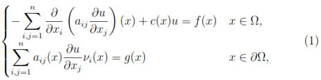
where aij, c  L∞(Ω), f L2(Ω), g L2(Ω), aij L∞(Ω) and ν is a unit normal vector to Ω.
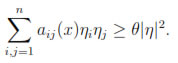
Here c(x) ≥ c1> 0 for all x Ω and A(x) = (aij(x))nxn is assumed to be uniformly elliptic in Ω, i.e. there exists θ > 0 such that for all x Ω and all η  n,
n,
After multiplying this differential equation by function v and using Green's formulas we find that:
B(u, v) = F(v)
with
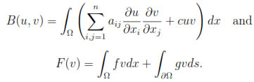
And this problem has a unique solution by the Lax-Milgram theorem.
We have used Neumann or flux boundary conditions here for simplicity; they are natural and do not need to be imposed explicitly. We expect that Dirichlet conditions could be implemented in this framework using, for instance, the Nitsche approach (See, perhaps, [6]). But, we do not pursue that here in order to focus on this new diffuse derivative approach.
We, further, expect that this approach could be extended to problems with higher order derivatives where the payoff in computational cost from the use of diffuse derivatives instead of full derivatives would be more pronounced.
3 Preliminaries on moving least squares (MLS)
3.1 The moving least squares method
Let Λ = {x1, x2, ..., xN} be a set of N distinct points inside and in the boundary of Ω  n which is an open and bounded set with Lipschitz boundary Ω and u1, u2, ...uN be the values of an unknown scalar function u(x) at the points in Λ (i.e. ui= u(xi), 1 ≤ i ≤ N ). Also let R > 0 (usually called dilation parameter) and consider a positive even weight function W(x) with compact support in
  and
and  W dx
W dx  1 Define WR(x) := W(x/R) and note WR has compact support in .
Let m << N and p(z) = {p0(z), p1(z), p2(z), ..., ps(z)}T be a basis of the subspace of polynomials of degree less or equal than m (denoted Pm) in n, placed in multi-index ordering. Note that s+1 = (n + m)!/(n!m!). For each x Ω consider
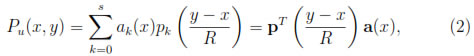
where a(x) = {a0(x), a1(x), a2(x), ..., as(x)}Tis chosen such that it minimizes the functional
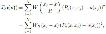
for a fixed x.
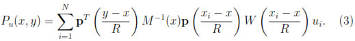
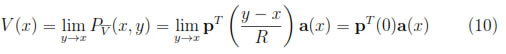
For each fixed x, Pu(x, y) is a polynomial in y of degree less than or equal to m that represents the best local approximation of u(x) for y in a small neighborhood of width 2R of x. Then, since the weight function W usually favors the points closer to x it is natural to define the following approximation of u(x):

A short calculation ([15]) shows that
a(x) = M-1(x)B(x)U,
where

and B(x) is a matrix whose ith column is p ((xi- x)/R) W ((xi- x)/R).
Thus,
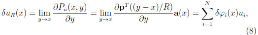
Therefore, letting y 7 x
x
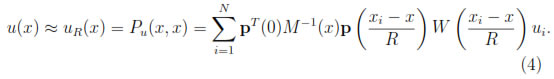
This expression can be written in the standard interpolation form
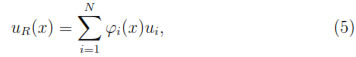
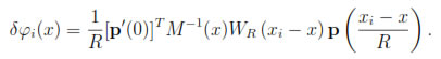
where φi(x), 1 ≤ i ≤ N, are called the shape functions and are given by
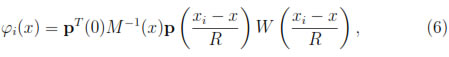
and uR(x) corresponds to the moving least squares approximation of the function u at the point x Ω.
Note also that from the minimization of functional J(a(x)) and, in computing the minimum via partial derivatives, the following orthogonality relationship holds:
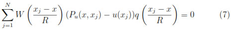
where q = q(z) is a polynomial of degree less than or equal to m.
3.2 Some error estimates for MLS approximations
We use the notation Wm,p(Ω) to denote the Sobolev space consisting of functions with m derivatives in Lp(Ω) (1 ≤ p ≤ ∞), and Hm(Ω) for the special case where p = 2. We use the following notation for the norms and seminorms:
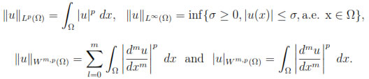
We will also denote  v := vL2(Ω).
The moving least squares method (MLS) has been used for the numerical solution of ordinary and partial differential equations in many papers, but very few of these include error estimates. The papers [9] and [8] provide such analysis and require the following properties:
(i) For each x Ω there exists at least s + 1 distinct points from Λ in  (x), where Lagrange interpolation is possible.
(ii) There exists c0> 0, independent of R, such that WR(z) ≥ c0 for all z (0).
(iii) There exists c# such that for all x Ω, card{xj BR(x), 1 ≤ j ≤ N } < c#.
(iv) For any x Ω there exists a constant cL such that the Lagrange basis functions associated with the set the points in property (i) are bounded by cL in B2R(x).
(v) WR C1(BR(0))  W1,∞(R) and there exists c1 > 0 such that
  WR(z)L∞(Rn) ≤ c1/R.
Note, in particular, that c0, c#, cL and c1 are independent of R and N. Here (iii) implies that card(Λ(x)) ≤ c#. Throughout the rest of this paper, C will denote a positive constant that is independent of R (and thus N as well).
Remark 3.1. In [8], Han and Meng stated that if conditions (ii) and (iv) are satisfied, then the family of particle distributions, Λ, is called regular, and it is enough to guarantee that there exists a constant L0 such that  M (x)-12≤ L0.
With these assumptions the following theorem was established (see proof in [9], [16], [8], [17], [15]):
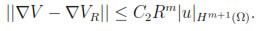
Theorem 3.1. If properties (i)-(v) hold and V Hm+1(Ω), then there exists a constant C1 that depends on c0, c#, cL and a constant C2 that depends on c0, c#, cL, c1 such that
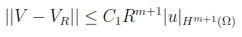
and
4 The diffuse derivative
Computation of the derivatives of a MLS function involves differentiation of a(x) which, in turn, involves differentiation of the M-1 and B matrices.
On the other hand, the derivative of polynomials in Pm is trivial and can be evaluated a priori. The concept of diffuse derivative, proposed in [3], exploits the fact that, for a MLS function u, Pu(x, y) is a good approximation of u = u(y) near the point x. Thus, in the one- dimensional case:
where
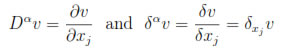
With obvious modifications for the multidimensional case, using multi-index notation. Below we indicate why u' (x)  δu(x). It can be shown (see [18]):
Proposition 4.1. Assume W(x) C0(n) and v(x) Cm+1(Ω) where Ω is a bounded open set in Rnwith Lipschitz boundary, and suppose sup(φi) is convex for each i. Then if m >  - 1,
- 1,

(where Dβv and δβv represent the full and diffuse derivatives, of order  β of v in multi-index notation).
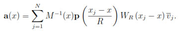
Now consider a function V VR= span{φ1, φ2, ..., φN} defined as
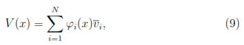
where  , 1 ≤ i ≤ N, are constants and φi(x) are the MLS shape functions. Note that V can also been written as
with
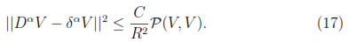
The analysis in [9] provides arguments to show that derivatives of the a(x) functions are small, which is crucial in our theory. The next lemma shows how the diffuse derivative is controlled by differences with the local MLS functional  (x, y). This lemma, somewhat of an inverse estimate, provides the key idea behind our stabilization.
Lemma 4.1. If properties (i)-(v) hold and α = 1 then there exists a constant C, independent of R, such that
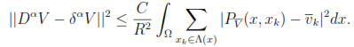
where Λ(x) = {xj Λ : x  .
.
Proof. Our proof follows very closely the proof of lemma 2.2 in [9] and Lemma 3 in [11].
Let α = (0,  , 0, αj, 0 , 0) n, α = 1. So
Let also, ej= jth unit vector in n.
A short calculation shows that
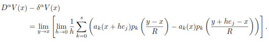
So,
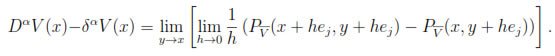
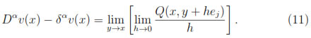
Define Q(x, y) := 
Notice that for each x, Q(x, y) is a polynomial in y of degree less or equal than m. Also, if z1, z2, ..., zs+1 are the points in BR/2(x) given by property (i), then using property (ii),
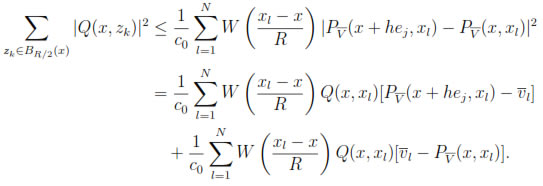
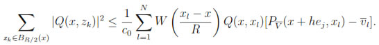
By the orthogonality property (7) the second term on the right hand side above is zero. Thus
By property (iv) and the Meanvalue theorem, we can guarantee that, for h small enough,  such that
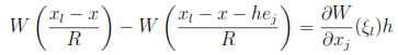
so,
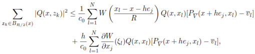
and using again the orthogonality condition (in x + hej) and property (v), we have
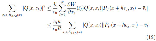
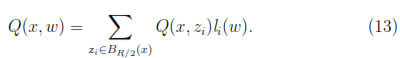
where Λ1+h(x) = {xk Λ : x - xk ≤ (1 + h)R}. On the other hand, we can use the Lagrange's polynomial basis functions l0, l1, . . . , ls, each of degree m at the s + 1 distinct points in BR/2(x) to write
So, using the Cauchy-Schwarz inequality,
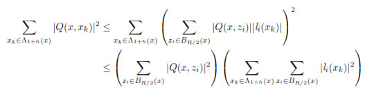
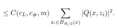
Using this result and Cauchy-Schwarz inequality in equation (12) we have
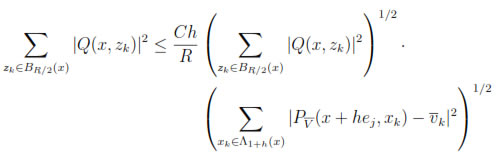
and thus,
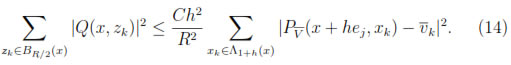
Using the equation (14), choosing z = y + hej and property (iv) in (13) we obtain, for all y BR(x) Ω,
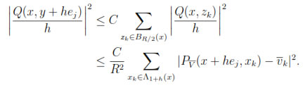
Finally, using this result in the equation (11) yields:
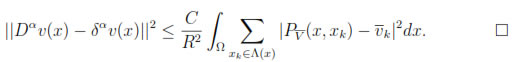
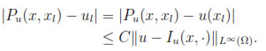
Remark 4.1. In the one dimensional case we presented in [15] and [11], we had that if V = uR(i.e. = ui= u(xi)) then Pu(x, ) is an interpolating polynomial of the function u at least on m + 1 distinct points in Λ(x); however, in the multidimensional case we are not aware of a similar result or whether this is true or not. Therefore, let us introduce for any x Ω the polynomial Iu(x, ) in Pm that interpolates u at the points that satisfy the property (i). We can prove the following theorem (see [9] or [15]):
Theorem 4.1. Let x Ω; if properties (i)-(iv) hold, then there exists a constant C depending only on c0, c#, cL such that for all y BR(x) Ω

Therefore, in particular taking y = x we have

5 A Galerkin Approximation Scheme
The stabilization of our Galerkin scheme will involve
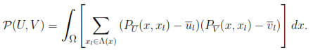
where U and V are MLS functions in VR as defined in (9). So, by lemma 4.1 we have
Let us also notice that from theorem 4.1 we have
Thus, by standard arguments from polynomial interpolation
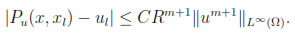
Hence,
For MLS functions u and w, the bilinear form for our Galerkin scheme is
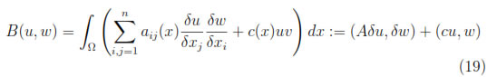
where
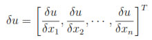
and A is a matrix whose ij entry is aij
So, our stabilized diffuse Galerkin method (SDGM) is as follows:
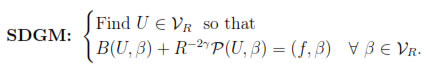
Here, we require γ > 0 and guidelines for it will be provided in the next theorem.

Remark 5.1. Note that SDGM is equivalent to the following Ritz-Galerkin formulation: Find U VR so that,

from which we can identify R-2γP (V, V), as a penalty or stabilization term.
We can now state and prove our main theorem:
Theorem 5.1. Let u Cm+1(Ω) be the exact solution of the equation (1), uR be its MLS approximation and U be the solution given by the numerical scheme SDGM, then if γ = m/2 + 1, there exists a constant C independent of R such that,

where
Proof. The proof of this theorem is similar to the proof of theorem 1 in [11].
First, for β 
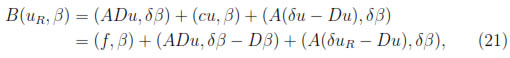
Now, let e = uR- U, then by the equations SDGM and (21) we have,
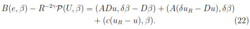
Now, choosing β = e we find
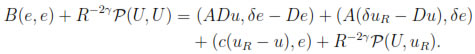
We can use the ellipticity condition to show
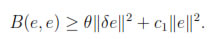
Therefore
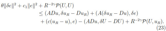
We can now use the Cauchy-Schwartz and arithmetic-geometric mean inequalities together with theorem 3.1 and proposition 4.1 to find
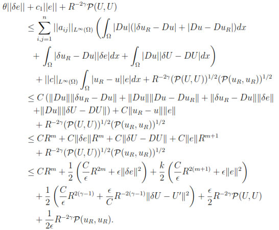
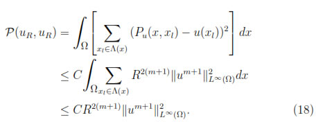
Now, by (18) and (17) we have
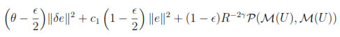
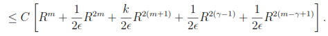
Choosing ε = 1/2, we conclude
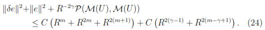
Then, taking γ = m/2 + 1 proves

and since P(U, U) ≥ 0 we find that

Combining this with proposition (4.1) we finish the proof.
6 Numerical results
In this section we present some numerical results on the convergence orders of the SDGM. The numerical results confirm the theoretical predictions.
Solutions are reported for the following numerical methods:
1. Diffuse element method (DEM).
2. Element free Galerkin method (EFG).
3. The stabilized diffuse Galerkin method (SDGM).
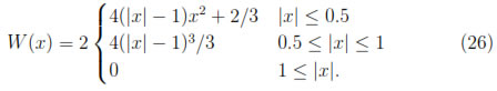
In all cases a background mesh of subintervals on cells was used for numerical integration. Within each integration cell, there was a set of Gauss-Legendre quadrature points. We kept the number of cells large enough so that numerical integration did not affect the convergence rates. The weight function was chosen to be the cubic spline:
We applied the numerical methods to the following boundary value problem:
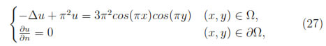
where Ω = [0, 1]x[0, 1] and n is the unit normal vector to the boundary of Ω. The exact solution of the equation (27) is u(x, y) = cos(πx)cos(πx).
For this example, we divide Ω into 11 x 11, 21 x 21 and 31 x 31 uniformly distributed points, and the dilation parameter (R/h) is kept constant for each m, so that the hypotheses from section 3 are satisfied.
Figures 1 and 2 show numerical results comparing EFG, DEM and SDGM for different dimensions (m) of the polynomial basis used in the MLS approximation. We report errors for both the numerical approximation of the solution of the equation (27) and the approximation of its first derivative with respect to x using diffuse derivatives, in the L2 norm. It is important to notice that similar results can be obtained for the full and diffuse derivatives with respect to y, and therefore for the gradient and diffuse gradient of u.
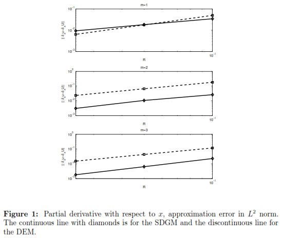
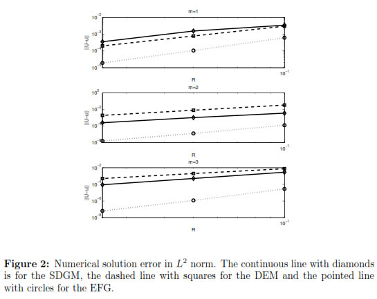
The convergence rates are summarized in tables 1 and 2. It can be seen that the numerical results suggest that for the SDGM

while we only get about u - U ≤ CR1.5 and δxu - δU ≤ CR0.5 for the DEM.
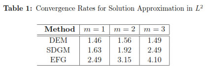
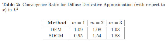
The numerical convergence rates are slightly better than our theoretical results on δxu - δxU and u - U, as is often true. We also observe that, in general, the errors obtained using SDGM are smaller than those using the standard DEM. The convergence rates for the DEM in the L2 norm are about 1.5 independent of the value of m and 1 for its derivative (similar observations were made in [19] and [11], although a small convergence rate for the DEM was obtained in the 1D case). Our SDGM performs better as m increases. Also, as expected the standard EFG gives the best convergence rates, but unfortunately it is very expensive from the computational point of view, which makes diffuse derivatives more attractive. It is important to notice that all these results agree with those found for the 1D case in [11].
Remark 6.1. A proof of the enhanced L2 convergence observed in the equation (28) remains an open question. The fact that our penalty term is not exactly zero at the true solution and integration by parts with diffuse derivatives is not possible, seem to make the standard duality argument impossible.
7 Conclusions
A modification to the traditional DEM, the stabilized diffuse Galerkin method (SDGM) has been proposed, in which a stabilization term is introduced to improve the overall accuracy and stability. The new scheme, like DEM, does not require the evaluation of full derivatives. This method is shown to give better results than DEM and converges to the true solution as the dilation parameter (R) goes to zero, or the order of the polynomial basis is increased, as demonstrated numerically and proved theoretically. The procedure described in this paper can be applied to more general multidimensional problems (see [15]).
We see SDGM as enhancing the viability of the diffuse derivative approach. Again, as suggested in Huerta et al [6], we think the versatility of the diffuse derivative could be helpful in fluid flows or mixed method computations.
Acknowledgements
We thank the University of Cincinnati and the Universidad Nacional de Colombia, for the support to this project . D. A. French was partially supported by a Charles Phelps Taft Summer Fellowship at the University of Cincinnati.
References
[1] T. Belytschko, Y. Krongauz, M. Fleming, D. Organ, and W. K. Liu, ''Smoothing and accelerated computations in the element free Galerkin method,'' J. Comput. Appl. Math, vol. 74, pp. 111-126, 1996. [ Links ] 54
[2] P. Breitkopf, A. Rassineux, G. Touzot, and P. Villon, ''Explicit form and efficient computations of MLS shape functions and their derivatives,'' Int. J. Numer. Meth. Engrg., vol. 48, pp. 451-466, 2000. [ Links ] 54
[3] B. Nayroles, G. Touzot, and O. Villon, ''Generating the finite element method: diffuse approximation and diffuse elements,'' Comput. Mech., vol. 10, pp. 307- 318, 1992. [ Links ] 54, 61
[4] T. Belytschko, Y. Y. Lu, and L. Gu, ''Element-free Galerkin methods,'' Int. J. Numer. Methods Engrg., vol. 37, pp. 229-256, 1994. [ Links ] 54
[5] Y. Krongauz and T. Belytschko, ''A Petrov-Galerkin diffuse element method (PG DEM) and its comparison to EFG,'' Computational Mechanics, vol. 19, pp. 327-333, 1997. [ Links ] 54
[6] A. Huerta, Y. Vidal, and P. Villon, ''Pseudo-divergence-free element free Galerkin method for incompressible fluid flow,'' Comput. Methods Appl. Mech. Engrg., vol. 193, pp. 1119-1136, 2004. [ Links ] 54, 57, 74
[7] I. Babuska, U. Banerjee, and J. Osborn, ''Survey of meshless and generalized finite element methods: A unified approach,'' Acta Numerica, pp. 1-125, 2003. [ Links ] 55
[8] W. Han and X. Meng, ''Error analysis of the reproducing kernel particle method,'' Comput. Methods Appl. Mech. Engrg., vol. 190, pp. 6157-6181, 2001. [ Links ] 55, 60
[9] M. Armentano, ''Error estimates in Sobolev spaces for moving least square approximations,'' SIAM J. Numer. Anal., vol. 39, pp. 38-51, 2001. [ Links ] 55, 60, 62, 66
[10] D. W. Kim and W. K. Liu, ''Maximum principle and convergence analysis for the meshfree point collocation method,'' SIAM J. Numer. Anal., vol. 44, pp. 515-539, 2006. [ Links ] 55
[11] D. A. French and M. Osorio, ''A Galerkin Meshfree Method with Diffuse Derivatives and Stabilization,'' Computational Mechanics., vol. 50, pp. 657-664, 2012. [ Links ] 55, 62, 65, 68, 73
[12] O. C. Zienkiewicz, ''Constrained variational principles and penalty function methods in the finite element analysis,'' Lecture Notes in Mathematics, vol. 363, pp. 207-214, 1974. [ Links ] 55
[13] T. Hughes, L. Franca, and G. Hulbert, ''A new finite element formulation for computational fluid dynamics: VIII. The Galerkin/least-squares method for advective-diffusive equations,'' Comput. Methods Appl. Mech. Engrg., vol. 73, pp. 173-189, 1989. [ Links ] 55
[14] S. Beissel and T. Belytschko, ''Nodal integration of the element-free Galerkin method,'' Comput. Methods Appl. Mech. Engrg., vol. 139, pp. 49-74, 1996. [ Links ] 55
[15] M. Osorio, ''Error analysis of a Meshfree method with diffuse derivatives and penalty stabilization,'' Ph.D. dissertation, University of Cincinnati, 2010. [ Links ] 58, 60, 65, 66, 74
[16] M. Armentano and R. Duran, ''Error estimates for moving least square approximations,'' Applied Numerical Mathematics, vol. 37, pp. 397-416, 2001. [ Links ] 60
[17] W. K. Liu and T. Belytschko, ''Moving least-square reproducing kernel methods. Part I: Methodology and convergence,'' Comput. Methods Appl. Mech. Engrg., vol. 143, pp. 113-154, 1997. [ Links ] 60
[18] D. Kim and Y. Kim, ''Point collocation methods using the fast moving least square reproducing kernel approximation,'' Int. J. Numer. Meth. Engrg., vol. 56, pp. 1445-1464, 2003. [ Links ] 61
[19] P. Breitkopf, A. Rassineux, and P. Villon, An introduction to moving least squares meshfree methods. In: Meshfree and particle based approaches in computational mechanics. Edited by P. Breitkopf and A. Huerta, 2004. [ Links ] 73
