


Services on Demand
Journal
Article
 English (pdf)
 Article in xml format
 Article references
 Send this article by e-mail
Indicators
-
 Cited by SciELO
 -
 Access statistics
Related links
-
 Cited by Google
 -
 Similars in
SciELO
Similars in
SciELO -
 Similars in Google
Share

 Permalink
Ingeniería y Ciencia
Print version ISSN 1794-9165
ing.cienc. vol.9 no.17 Medellín Jan./June 2013
ARTÍCULO ORIGINAL
A Fully Discrete Finite Element Scheme for the Derrida-Lebowitz-Speer-Spohn Equation
Un esquema de elementos finitos completamente discreto para la ecuación de Derrida-Lebowitz-Speer- Spohn
Jorge Mauricio Ruiz Vera1 and Ignacio Mantilla Prada2
1 Doctor en Ciencias Matemáticas, jmruizv@unal.edu.co, Departamento de matemáticas, Universidad Nacional de Colombia, Bogotá, Colombia.
2 Dr. rer. nat. in Mathematik, imantillap@unal.edu.co, Departamento de matemáticas, Universidad Nacional de Colombia, Bogotá, Colombia.
Received:07-12-2012, Acepted: 05-03-2013
Available online: 22-03-2013
MSC: 35G25, 65M60, 82D37
Abstract
The Derrida-Lebowitz-Speer-Spohn (DLSS) equation is a fourth order in space non-linear evolution equation. This equation arises in the study of interface fluctuations in spin systems and quantum semiconductor modelling. In this paper, we present a finite element discretization for a exponential formulation of a coupled-equation approach to the DLSS equation. Using the available information about the physical phenomena, we are able to set the corresponding boundary conditions for the coupled system. We prove existence of the discrete solution by fixed point argument. Numerical results illustrate the quantum character of the equation. Finally a test of order of convergence of the proposed discretization scheme is presented.
Key words: Finite elements, Nonlinear evolution equations, Semiconductors.
Highlights
• Exponential formulation of a coupled-equation approach to the DLSS equation. • Existence proof of the discrete solution by means of a fixed point argument. • Numerical results suggest optimal convergence of the method in the H1(Ω)-norm.
Resumen
La ecuación de Derrida-Lebowitz-Speer-Spohn (DLSS) es una ecuación de evolución no lineal de cuarto orden. Esta aparece en el estudio de las fluctuaciones de interface de sistemas de espín y en la modelación de semicoductores cuánticos. En este artículo, se presenta una discretización por elementos finitos para una formulación exponencial de la ecuación DLSS abordada como un sistema acoplado de ecuaciones. Usando la información disponible acerca del fenómeno físico, se establecen las condiciones de contorno para el sistema acoplado. Se demuestra la existencia de la solución discreta global en el tiempo via un argumento de punto fijo. Los resultados numéricos ilustran el carácter cuántico de la ecuación. Finalmente se presenta un test del orden de convergencia de la discretización porpuesta.
Palabras clave: Elementos finitos, Ecuaciones no lineales de evolución, Semiconductores.
1 Introduction
The Derrida-Lebowitz-Speer-Spohn (DLSS) equation is a nonlinear fourth order parabolic equation which was proposed to study the interface fluctuations in a spin system [1], [2]. Coincidentally, in the mathematical modelling of the charge transport in quantum semiconductor devices the DLSS equation appears as the zero temperature and zero electric field quantum drift diffusion equation [3].
In this paper, we discuss a new numerical technique to solve the DLSS equation
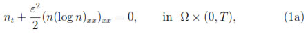
subject to the initial and boundary conditions
where n0 is a given function, Ω is the bounded interval (0, 1), and T > 0 is a fixed positive time. Regarding semiconductor modelling, n(x, t) denotes the electron concentration, and ε is the scaled Planck constant; it is of order O(10-2;...;-4). The Dirichlet boundary conditions (1c) model charge neutrality at the boundary contacts, while Neumann boundary conditions (1d) describe no current flow passing through the boundary.
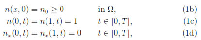
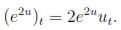
Due to the several difficulties and challenges that fourth order differential equations have (see e.g. [4]), several researchers have analyzed the problem (1). For instance, existence results of a positive classical solution locally in time and nonnegative solutions globally in time of (1) are found in [1] and [5] respectively. More recently, in [6] the existence of the solution for the multidimensional equation is proven. Furthermore, in [7], [8] and [9] the long-time behavior of solutions is studied. However, concerning its numerical solution not much work is known. In [1] and [5] a fully implicit finite difference discretization scheme was employed to the equivalent formulation
in order to verify thepreservation of the non negativity by the solution n. An alternative numerical treatment is presented in [10], where a fully discrete variant of the minimizing movement scheme is developed based on the particular structure of (1a). The numerical experiments in [10] suggest that this scheme is unconditionally stable and second-order convergence.
With this paper, we pursue a different numerical approach based on the following two main steps: First, in order to guarantee the positivity of the solution n, we perform an exponential transformation of variable n = e2u. Such transformation has been already used in [5] and [8] for theoretical purposes but not for numerical tasks. After that, we introduce a new variable w = -ε2e2uuxx in order to write Equation (1) as two coupled partial differential equations, which require less stringent smoothness constrains over the solution as well as for the finite elements approximation than consider the single fourth order equation. Finally, the resulting problem is discretized by a fully discrete finite element scheme.
The paper is organized as follows. In section 2 we present a coupled equation decomposition after an exponential transformation of variables for DLSS equation and discuss the corresponding boundary conditions in the context of the quantum charge transport in semiconductors. We formulate the fully discrete finite element scheme and numerical treatment of the nonlinearities in section 3. Existence of the discrete solution is proved in 3.1. Finally, section 4 is devoted to the numerical results. Concluding remarks are given in section 5.
2 Exponential and coupled equation formulation
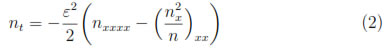
It is well known, that for a fourth order differential equation the nonnegativity of the initial data does not imply the same property of solutions at any time. This motivated us to perform the change of variable n = e2u, which yields the following exponential form of problem (1)
Such formulation of (1) has been proposed in [5] as a crucial step to prove the existence of nonnegative weak solutions, but it has not been used for finding an approximate solution of (1). In fact, in [5] it was ∫proved that, if the initial condition u0 is a measurable function such that Ω(exp(2u0)-2u0)dx < ∞, then problem (3) has a solution u 
 (Ω). Furthermore, note that the existence of positive solution n of the problem (1) is a consequence of the existence solution u of (3).
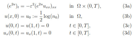
In order to relax the smoothness constrains on the solution as well as the finite element approximation, we introduce an auxiliary variable w = -ε2e2uuxx. Then we may write problem (3) as a coupled second order system of a nonlinear parabolic and nonlinear elliptic equations
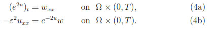
Now, we state the corresponding boundary conditions. For the unknown u it is easy to see that conditions (3c) and (3d) hold. However the values of w or wx at the boundary can not be derived straightforwardly, hence we need to consider additional information about the electron transport at the boundary. For this purpose, let us assume smooth non vacuum solutions (n  0) of (1a), then
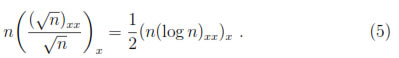
In addition, from [11] it is known that the quantum current has to vanish at the semiconductors contacts, that is
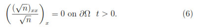
Combining (5) with (6) and taking n = e2u we obtain
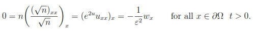
This lead us to impose homogeneous Neumann conditions for w(x, t) i.e,

Remark 2.1. The differential operator ( )xx/ is the so called Bohm potential and appears as the quantum correction term of the classical drift-diffusion model for semiconductors [3], [12].
3 Numerical discretization
In this section we describe the construction of finite element method for the coupled system of nonlinear partial differential Equation (4) with boundary conditions (3c) and (7). To give a variational formulation of this boundary value problem, we introduce the spaces
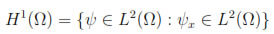
and

Now we multiply (4a) and (4b) by Φ  (Ω) and ψ H1(Ω) respectively and integrating by parts over Ω, we find that
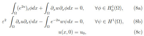
since wx(0, t) = wx(1, t) = 0 and ux(0, t) = ux(1, t) = 0 for all t ≥ 0.
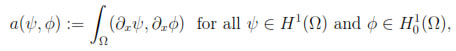
If ( , ) denotes the L2(Ω) inner product and the mapping a(, ) : H1(Ω) x (Ω)
 is defined by
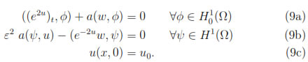
then the variational formulation of (4) with boundary condition (3c) and (7) is: Find the pair (w, u)(t) H1(Ω) x (Ω) for all t (0, T) such that
In order to discretize (9) in time, first we apply the chain rule to the time derivative term in (9a), then
Next, we divide the interval (0, T] into M equal parts, i.e. time step τ = T/M, and each time level tk = kτ , with k = 0, 1, .., M. Then we approximate the quantity ut by finite difference. After that, if the index k signifies the most recent known time level, then evaluating the non linear term e2u at the time level k and the spatial terms at the next unknown time level k + 1 produces the semi-discrete problem: Find the pair (wk+1, uk+1) H1(Ω) x (Ω) for k = 0, ..., M - 1 such that
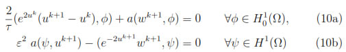
with u0 = u0.
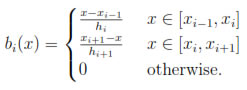
We now discretize also in space, let 0 = x0 < x1 < ... < xN = 1 be mesh on the interval Ω = (0, 1) with hi := xi - xi-1, i = 1, ..., N. In addition, let Wh  H1(Ω) be the corresponding subspace of continuous piecewise linear functions on Ω and Vh (Ω) be the subspace of continuous piecewise linear functions on Ω vanishing at x = 0 and x = 1. Furthermore, let us equip Vh and Wh with a basis
  and
and  respectively, where
Then for any  Wh and
  Vh, these can be written as (x) =
 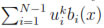 and
and 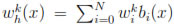 in the k-th time level. We now approximate the nonlinear terms in (10a) and (10b) by their linear interpolants on the mesh, that is
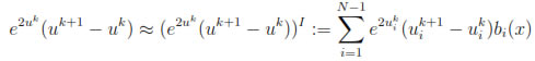
and
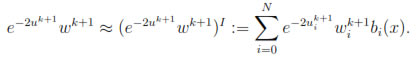
Therefore, the fully finite element method for (9) reads as follows: Find for k = 0, ..., M - 1, the pair  Wh x Vh such that
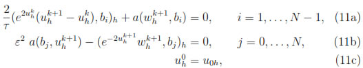
where (f, g)h := (fI, g).
Finally, computing the integrals exactly in system of Equations (11a)- (11b), we obtain the nonlinear system of equations
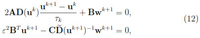
where the vectors uk+1 N-1 and wk+1 N+1 contain the nodal unknowns  (t) and
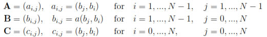
  (t) respectively. The matrices A,B,C are given by
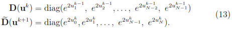
while the diagonal matrices D(uk) and  (uk+1) are
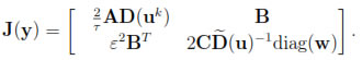
In order to solve the nonlinear system (12), let us denote by y 2N the unknown vector  and employ the Newton method
y(m+1) = y(m) + Δy
where Δy is the solution of the linear system
J(y(m)) Δy = -F(y(m))
with F(y) : 2N 2N given by (12) and Jacobi matrix
We choose y(0) =  as a initial guess for the Newton iteration, provided that the time step τ is small enough.
3.1 Existence of the discrete solutions
In this section, we prove the existence of the discrete solution by means of a fixed point argument.
First, let us observe that from the symmetric positive definiteness of matrices A and D(z) with given z N-1, the bilinear form on N-1 defined by

is an inner product on N-1.
Theorem 3.1. The nonlinear system of Equations (12), has a solution.
Proof: Since the mass matrices A and C are symmetric positive definite and the terms e±ui(t) 0 for i = 0, 1, ..., N in (13), we are able to eliminate the unknown w from the second Equation of (12). Then we may write (12) as the Equation G(uk+1) = 0 for each time level k, where G is a continuous function from N-1 to N-1 given by

Let us now introduce the inner product on N-1 defined by
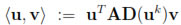
for a given uk. Hence, it defines a norm  D equivalent to the usual euclidian norm in N-1. Further, we define the ball BR(0) := {u N-1 : uD ≤ R} with R = ukD. Then

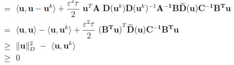
for all u such that uD ≥ R. Therefore, by the Minty-Brower's fixed point theorem [13], G(u) has a solution in BR(0).
Remark 3.1. We observe that it is possible to solve the nonlinear system of Equations G(uk+1) = 0 by Newton's method instead of (12). However, the presence of the inverse matrices of A and C yields a loss of sparseness of the Jacobi matrix of G(u). Hence, it is not computationally efficient to solve such equation even though it has N - 1 unknowns.
4 Numerical results
To demonstrate the efficacy of the finite element described before, we consider the fourth-order nonlinear parabolic problem (1) with nonnegative initial condition
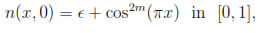
for m = 1, 8 and ε = 10-6. Further we give a physical interpretation of the results as well as an experimental error convergence analysis for the proposed spatial discretization.
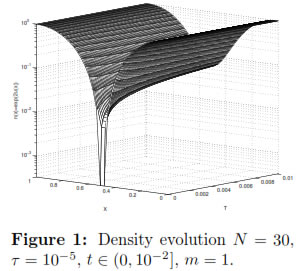
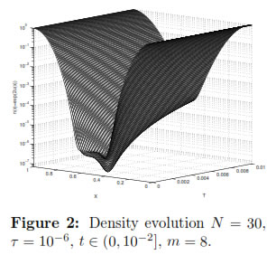
We apply the fully finite element method (11) for solving the problem (1) up to T = 10-2. Since the method is semi-implicit, we choose τ ≤  to keep it stable. We present in Figure 1 numerical results for m = 1 with space discretization step h = 1/30, and time step τ = 10-5 and in Figure 2 for m = 8 with space discretization step h = 1/30, and time step τ = 10-6. In each time step we have solved the nonlinear system of Equations (12) by means of the Newton's method (See section 3).
4.1 Physical interpretation of the solution
Physical processes modelled by fourth order parabolic equations are very similar to the diffusion phenomena but the oscillatory data is damped more rapidly. Indeed, from Figure 1 we observe that at the instant t = 0 there is high concentration of electron on the boundaries x = 0, x = 1 and it decrease in the interior of the semiconductor until reach the zero at x = 0.5. Then, the electrons move from the higher concentration parts to the lower concentration part. This movement finishes when the distribution of electrons in the semiconductor is almost uniform, i.e the steady state is reached t = t∞. In contrast, when m = 8 the electron density evolution does not behave like classical diffusion (Figure 2).
In this case the initial electrons density is very low in a neighborhood of x = 0.5, hence the electrons diffuse to this low density region and move almost freely, without many collisions, during some period of time. As a consequence, they start to accumulate in the center of the semiconductor (see the small peak at t = 2x10⁻⁴) leaving two areas with lower density. Afterwards, the electrons are redistributed rapidly, vanishing the peak. Then, the situation behaves like in the case m = 1. Such behavior on the electron density gives an evidence of the quantum effect due to the Bohm potential.
Similar behaviors for the electron density n have been obtained in [1], [5] and [10]. However, in [5] Equation (2) is solved for the variable n using a finite difference scheme, while we solve (1a) for the variable u =  log(n).
4.2 Convergence rates
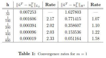
In order to examine the convergence properties with respect to the spatial step size h, we use a solution û on a very fine grid (h = 1/1600) as a reference solution in computing the approximation errors in the L2(Ω)- norm and H1(Ω)-norm. Furthermore, we solved the system (4) on five grids with sizes h = 1/(2k 50), k = 0, . . . , 4. Let  denote the numerical solution corresponding to the space grid with size h at final time t = T and let ûh be the restriction of the fine grid solution to the h-grid, so that we can define the approximate error e(h) =
  . Since we expect that the method is r'th order accurate, that is e(h)
  Chr as h 0, then the convergence order r can be estimated as
r log2 (e(h)/e(h/2)).
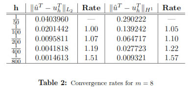
Table 1 presents for various space step sizes, numerical errors for and convergence rates when m = 1. One can see from the table optimal orders of convergence in the L2(Ω)-norm and H1(Ω)-norm. On the other hand, Table 2 shows numerical results for m = 8 where the L2(Ω)-norm of the error decreases to order one; while the H1(Ω)-norm error remains to be first ordert
5 Conclusions
In this paper we have presented a new numerical approach for a fourth order nonlinear problem based on piecewise linear finite element method. We applied a semi implicit discretization in time to construct the fully discrete solution and prove the existence of the fully finite element discrete solution. Due to the used exponential transformation of variables, the proposed method guarantee the positivity of the solution. Numerical calculations show that the proposed scheme is convergent but it has only an optimal convergence rate in the H1(Ω)-norm. Future work will focus on a consistency analysis of the proposed method.
Acknowledgments
The authors would like to thank the anonymous referees for several suggestions for the improvement of this paper.
References
[1] P. M. Bleher, J. L. Lebowitz, and E. R. Speer, ''Existence and positivity of solutions of a fourth-order nonlinear PDE describing interface fluctuations,'' Communications on Pure and Applied Mathematics, vol. 47, no. 7, pp. 923- 942, 1994. [ Links ] 98, 99, 108
[2] B. Derrida, J. L. Lebowitz, E. R. Speer, and H. Spohn, ''Fluctuations of a stationary nonequilibrium interface,'' Phys. Rev. Lett., vol. 67, pp. 165-168, July 1991. [ Links ] 98
[3] R. Pinnau, ''The Linearized Transient Quantum Drift Diffusion Model-Stability of Stationary States,'' ZAMM - Journal of Applied Mathematics and Mechanics / Zeitschrift für Angewandte Mathematik und Mechanik, vol. 80, no. 5, pp. 327- 344, 2000. [ Links ] 98, 101
[4] L. L. A. Peletier and W. C. Troy, Spatial Patterns: Higher Order Models in Physics and Mechanics. Progress in Nonlinear Differential Equations and Their Applications Series, Boston: Springer, 2001. [ Links ] 99
[5] A. Jüngel and R. Pinnau, ''Global Non-Negative Solutions of a Nonlinear Fourth- Order Parabolic Equation for Quantum Systems,'' 2000. [ Links ] 99, 100, 108
[6] A. Jüngel and D. Matthes, ''The Derrida-Lebowitz-Speer-Spohn equation: Existence, NonUniqueness, and Decay Rates of the Solutions,'' SIAM Journal on Mathematical Analysis, vol. 39, no. 6, pp. 1996-2015, 2008. [ Links ] 99
[7] M. J. Cáceres, J. A. Carrillo, and G. Toscani, ''Long-Time Behavior for a Nonlinear Fourth-Order Parabolic Equation,'' Transactions of the American Mathematical Society, vol. 357, no. 3, pp. 1161-1175, 2005. [ Links ] 99
[8] M. Pia Gualdani, A. Jüngel, and G. Toscani, ''A Nonlinear Fourth order Parabolic Equation with Nonhomogeneous Boundary Conditions,'' SIAM Journal on Mathematical Analysis, vol. 37, no. 6, pp. 1761-1779, 2006. [ Links ] 99
[9] A. Jüngel and G. Toscani, ''Exponential time decay of solutions to a nonlinear fourth-order parabolic equation,'' Zeitschrift für angewandte Mathematik und Physik ZAMP, vol. 54, no. 3, pp. 377-386, 2003. [ Links ] 99
[10] B. Düring, D. Matthes, and J. P. Milisic, ''A gradient flow scheme for nonlinear fourth order equations,'' Discrete and Continuous Dynamical Systems - Series B (DCDS-B), vol. 14, no. 3, pp. 935 - 959, 2010. [ Links ] 99, 108
[11] R. Pinnau, ''A note on boundary conditions for quantum hydrodynamic equations,'' Applied Mathematics Letters, vol. 12, no. 5, pp. 77-82, 1999. [ Links ] 101
[12] M. G. Ancona and H. F. Tiersten, ''Macroscopic physics of the silicon inversion layer,'' Phys. Rev. B, vol. 35, pp. 7959-7965, May 1987. [ Links ] 101
[13] E. Zeidler, Nonlinear Functional Analysis and Its Applications II/A. Berlin: Springer-Verlag, 1 ed., 1990. [ Links ] 106
