


Services on Demand
Journal
Article
 English (pdf)
 Article in xml format
 Article references
 Send this article by e-mail
Indicators
-
 Cited by SciELO
 -
 Access statistics
Related links
-
 Cited by Google
 -
 Similars in
SciELO
Similars in
SciELO -
 Similars in Google
Share

 Permalink
Ingeniería y Ciencia
Print version ISSN 1794-9165
ing.cienc. vol.9 no.17 Medellín Jan./June 2013
ARTÍCULO ORIGINAL
A Fully-Discrete Finite Element Approximation for the Eddy Currents Problem
Un esquema completamente discreto basado en elementos finitos para el problema de corrientes inducidas
Ramiro Acevedo1 and Gerardo Loaiza2
1 Doctor en Ingeniería Matemática, rmacevedo@unicauca.edu.co, Universidad del Cauca, Popayán, Colombia.
2 Magíster en Ciencias Matemáticas, gloaiza@unicauca.edu.co, Universidad del Cauca, Popayán, Colombia.
Received: 18-04-2012, Acepted: 10-12-2012
Available online: 22-03-2013
MSC:78M10, 65N30
Abstract
The eddy current model is obtained from Maxwell's equations by neglecting the displacement currents in the Ampère-Maxwell's law. The so-called ''A, V - A potential formulation'' is nowadays one of the most accepted formulations to solve the eddy current equations numerically, and Bíró & Valli have recently provided its well-posedness and convergence analysis for the time-harmonic eddy current problem. The aim of this paper is to extend the analysis performed by Bíró & Valli to the general transient eddy current model. We provide a backward-Euler fully-discrete approximation based on nodal finite elements and we show that the resulting discrete variational problem is well posed. Furthermore, error estimates that prove optimal convergence are settled.
Key words: Transient eddy current model, potential formulation, fully-discrete approximation, finite elements, error estimates.
Highlights
• We have proposed a fully-discrete finite element approximation for the eddy current problem. • The eddy current problem is considered in a bounded domain, without topological restrictions on the conductor. • We have shown that at each step the fully-discrete scheme propose is well posed. • We have obtained quasi-optimal error estimates of the typical physical variables of interest of the eddy current problem.
Resumen
El modelo de Eddy Current se obtiene a partir de las ecuaciones de Maxwell, despreciando las corrientes de desplazamiento de la Ley de Ampère-Maxwell. Bíró & Valli realizaron recientemente el análisis de existencia y unicidad de solución y el análisis teórico de convergencia para una de las formulaciones más populares del problema de Eddy Current en regimen armónico, conocida como ''formulación en potenciales A, V - A''. En el presente artículo se extiende el análisis realizado por Bíró & Valli al modelo evolutivo general de Eddy Current. Presentamos un esquema completamente discreto para la formulación, basado en una aproximación temporal usando un método de Euler implícito y una aproximación espacial a través del método de elementos finitos. Además, demostramos que el problema discreto resultante es un problema bien planteado y obtenemos estimaciones del error que muestran convergencia óptima.
Palabras clave: Modelo evolutivo de Eddy Current, formulación en términos de potenciales, esquema completamente discreto, elementos finitos, estimaciones de error.
1 Introduction
In applications related to electrical power engineering (see for instance [1]) the displacement currents existing in a metallic conductor are negligible compared to the conduction current. In such situations the displacement currents can be dropped from Maxwell equations to obtain a magneto-quasistatic submodel usually called eddy current problem ; see for instance [2, Chapter 8]. From the mathematical point of view, this submodel provides a reasonable approximation to the solution of the full Maxwell system in the low frequency range [3].
Among the numerical methods used to approximate eddy current equations, the finite element method (FEM) and methods combining FEM and boundary element method (FEM-BEM) are the most extended, see, for instance, the recent book by Alonso & Valli [4] for a survey on this subject including a large list of references. In the applied mathematical literature, we can find several recent papers devoted to the numerical analysis of the 3D time dependent eddy current model, in bounded domains as well as in unbounded domains by using FEM and FEM-BEM methods: Meddahi & Selgas [5], Ma [6], Acevedo et al. [7], Kang & Kim [8], Prato et al. [9], Acevedo & Meddahi [10], Bermudez et al. [11], Camaño & Rodríguez [12]. The main differences among these works are the selected unknowns to compute the electromagnetic field, the topological assumptions on the conductor domain and the boundary conditions when the problem is solved in a bounded domain.
The aim of this paper is to analyze a finite element fully-discrete approximation for the time-dependent eddy current problem in a bounded domain, based in a formulation in terms of a vector magnetic potential and an electric scalar potential. Numerical experiments showing the efficiency of this approach, were reported by Bíró & Preis (1989) [13], and nowadays, it is the basis of several commercial codes to compute the solution of the eddy current model. Bíró & Valli (2007) [14] have studied that potential formulation for the time-harmonic eddy current model and have proved its well-posedness and theoretical convergence in a general geometric situation. However, a similar analysis for the transient case has not been realized yet. Although, Kang & Kim (2009) in [8] have recently provided quasi-optimal error estimates, showing the theoretical convergence of the method in the case of a simply-connected conductor and by assuming homogeneous conditions for the electromagnetic fields on the boundary of the conductor, these assumptions are very restrictive for many real applications (e.g., metallurgical electrodes [15] and power transformers [16]). Moreover, the decay conditions on the fields at infinity (see [3]) allow to assume that the electromagnetic field is weak far away from the conductor and not on its boundary, as it was assumed by Kang & Kim when the artificial homogeneous boundary conditions are supposed.
In order to improve the results obtained by Kang & King for more realistic applications, we consider a multiply-connected conductor and we opt for a typical approach: to restrict the eddy current equations to a sufficiently large computational domain containing the region of interest and impose a convenient artificial homogeneous boundary conditions for the electromagnetic fields on its border. We provide a backward-Euler fully-discrete approximation based on nodal finite elements to approximate the solution of the resultant model. This fully-discrete scheme solves in each time an elliptic problem and we use the techniques used in [14] and [17] to prove the ellipticity of its bilinear form. Furthermore, by using this ellipticity we define projection operators to the discrete finite element subspaces and obtain quasi-optimal error estimates, which allows us to approximate the typical physical variables of interest of the eddy current problem: the eddy currents in the conductor and the magnetic induction in the computational domain.
The outline of the paper is as follows: In section 2, we summarize some results concerning tangential traces in H(curl; Ω) and recall some basic results for the study of time-dependent problems. In Section 3, we introduce the eddy current model in a bounded domain and deduce a potential-based formulation (the so-called ''A, V - A potential formulation'') for the time-dependent eddy current problem. In Section 4, we obtain a variational formulation for the problem and its fully-discrete approximation scheme is analyzed in Section 5. Finally, the results presented in Section 6 prove that the resulting fully discrete scheme is convergent in an optimal way. We end this paper by summarizing its main results in Section 7.
2 Preliminaries
We use boldface letters to denote vectors as well as vector-valued functions and the symbol 
 represents the standard Euclidean norm for vectors. In this section Ω is a bounded open set in
  3 with a Lipschitz boundary. We denote by Γ its boundary and by n the unit outward normal to Ω. Let
be the inner product in L2(Ω) and  0,Ω the corresponding norm. As usual, for all s > 0, s,Ω stands for the norm of the Hilbertian Sobolev space Hs(Ω) and s,Ω for the corresponding seminorm. The space H1/2(Γ) is defined by localization on the Lipschitz surface Γ. We denote by 1/2,Γ the norm in H1/2(Γ) and { , }Γ stands for the duality pairing between H1/2(Γ) and its dual H-1/2(Γ). Let γ : H1(Ω)
  H1/2(Γ) and γ : H1
 H1/2(Γ)3be the standard trace operator acting on scalar and vector fields respectively. In what follows we use φΓ and φΓ to denote γ(φ) and γ(φ) for any φ
  H1(Ω) and φ H1respectively.
2.1 Normal and tangential traces
We recall that

endowed with the norm vH(div;Ω):=  is a Hilbert space and that C∞ is dense in H(div; Ω). By using this density result, the mapping γn: C∞ L2(Γ) given by v 7 γn(v) := vΓn, can be extended by continuity to define the normal trace operator (see, for instance, [18, Theorem 3.24])
which is bounded, surjective and possesses a right inverse. Moreover, the following Green's identity holds for any v H(div; Ω) and φ H1(Ω)

where, as usual, v n denotes γn(v). Furthermore, we denote by H0(div; Ω) the kernel of γn in H(div; Ω), i.e.,

We also recall that

endowed with the norm endowed with the standard norm in L2(Γ)3. We define the tangential trace γτ:C∞ The spaces Let us notice that the density of H1/2(Γ)3 in L2(Γ)3 ensures that vH(curl;Ω):=  is a Hilbert space and that C∞ is dense in H(curl; Ω) (see, for instance, [18, Theorem 3.26]). Tangential traces of functions in H(curl; Ω) are also understood even in the case of polyhedral domains thanks to the recent results given by Buffa & Ciarlet [19, 20] and Buffa, Costabel & Sheen [21]. We give here a brief summary of these fundamental tools. We begin by considering the space
  L2τ (Γ) and the tangential component trace πτ:C∞
  as γτv:= vΓxn and πτv:= n x (vΓ x n) respectively. The previous traces can be extended by continuity to H1.
 := γτ(H1) and
  := πτ (H1), are respectively endowed with the Hilbert norms
 and are dense subspaces of L2τ (Γ). The dual spaces of and with as pivot space, are denoted by
  and
and  respectively.
By using the density of C∞in H(curl; Ω) and the well known Green's formula (see, for instance, [18, Corollary 3.20])

it is easy to deduce that γτ and πτ can be extended to define bounded tangential mappings from H(curl; Ω) onto onto respectively. The space H0(curl; Ω) stands for the kernel of γτ in H(curl; Ω), i.e.,

where, as usual, vΓ x n denotes γτv.
The ranges of γτ and πτ are characterized in the following result. We refer to [19, 21] for the definition of the differential operators divΓ and curlΓ on piecewise smooth Lipschitz boundaries.
Theorem 2.1. Let

and

Then
 are surjective and possess a continuous right inverse.
The spaces H-1/2 (divΓ; Γ) and H-1/2 (curlΓ; Γ) are dual to each other, when is used as pivot space, i.e., the usual -inner product can be extended to a duality pairing { , }τ,Γ between H-1/2 (divΓ; Γ) and H-1/2 (curlΓ; Γ). Moreover, the following Green's identity holds true

Proof. See Theorem 4.1 and Lemma 5.6 of [21].

Since in the eddy current problem the physical domain requires to be split into two non-overlapping domains: the conductor and the insulator domain (see Section 3.1 below), we end this subsection by recalling the following classical result that will be used often in the rest of the paper.
Lemma 1. Assume Ω is split into two parts Ω =  1
1 2, where Ω1 and Ω2 are two non-overlapping Lipschitz domains. Let Σ :=
  Ω1
Ω1  Ω2 be the interface between the two subdomains and let ν be a unit normal to Σ.
a) A function v belongs to H(div; Ω) if and only if its restrictions vΩ1 and vΩ2 belong to H(div; Ω1) and H(div; Ω2), respectively, and
b) A function v belongs to H(curl; Ω) if and only if its restrictions vΩ1 and vΩ2 belong to H(curl; Ω1) and H(curl; Ω2), respectively and

Proof. See, for instance, [18, Lemma 5.3].
2.2 Basic spaces for time dependent problems
Since we will deal with a time-domain problem, besides the Sobolev spaces defined above, we need to introduce spaces of functions defined on a bounded time interval (0, T) and with values in a separable Hilbert space V, whose norm is denoted here by V. We use the notation C0([0, T]; V) for the Banach space consisting of all continuous functions f : [0, T] V. More generally, for any k  , Ck([0, T]; V) denotes the subspace of C0([0, T]; V) of all functions f with (strong) derivatives of order at most k in C0([0, T]; V), i.e.,

We also consider the space L2(0, T; V ) of classes of functions f : (0, T) V that are Böchner-measurable and such that
Furthermore, we will use the space
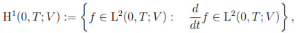
where  is the (generalized) time derivative of f; see, for instance, [22, Section 23.5].
3 The model problem
3.1 Eddy current problem
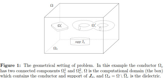
We consider a standard eddy current problem: to determine the electromagnetic fields induced in a three-dimensional conducting domain by a given source time-dependent compactly-supported current density. The eddy current problem is in principle posed in the whole space. However, we restrict it to a bounded computational domain containing both, the conductor and the support of the source current, such that adequate boundary conditions can be imposed on its boundary. To this aim, we choose the geometry of the computational domain as simple as possible (e.g., simply connected with a connected boundary).
Let Ωc  3 be the conducting domain and let us assume that it is an open and bounded set with boundary Γc. Let Ω 3 be a simply connected bounded domain with a connected boundary Γ, such that c Ω. We suppose that both, Ω and Ωc are Lipschitz domains and we denote by n and nc the outward unit normal vectors to Ω and Ωc, respectively. Let Ωd:= Ω \ c be the subdomain of Ω occupied by dielectric material, which includes the support of the source current Jd (see Figure 1).
The electric and magnetic fields E : Ωc x [0, T] 3 and H : Ω x [0, T] 3 are solutions of a submodel of Maxwell's equations obtained by neglecting the displacement currents (see, for instance, [13]):
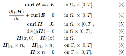
Let us remark that because of H(, t) must belong to H(curl; Ω) a.e. in [0, T], Lemma 1 implies the magnetic field has to satisfy the coupling conditions, Equation (8).
The magnetic permeability µ and the conductivity σ are bounded functions satisfying:
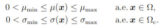
The data of the problem are the source current density Jd L2(0, T; L2), for which we assume for a.e. t (0, T)

and the initial magnetic field H0 H(curl; Ω).
3.2 The A, V - A potential formulation
We now recall a classical formulation of the eddy current problem in terms of two potentials: a magnetic vector potential A and an electric scalar potential V. We refer to Bíró & Preis [13] for a detailed discussion, which also includes numerical tests showing the efficiency of this approach.
In order to introduce the magnetic vector potential, we notice that, by using [23, Theorem I.3.5.], Equation (6) implies that there exists a unique A L2(0, T; H(curl; Ω)) such that
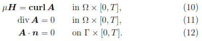
We notice that from (8) and (10) it follows that
Moreover, since A L2(0, T ; H(curl; Ω)), from Lemma 1 and Equation (11) we have
Next, according to Bíró & Preis [13] (see also Bíró & Valli [14]) we introduce an electric scalar potential V : Ωc x [0, T] , such that
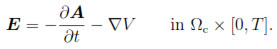
If we define
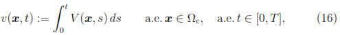
we obtain
Hence, from (3) there follows that
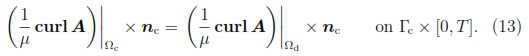
Moreover, since H(, t) H(curl; Ω) a.e. t in [0, T], we have curl H(, t) H(div; Ω) a.e. t in [0, T], and consequently, from Lemma 1 we have

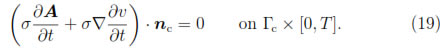
Then, from (3), (5) and recalling that suppJd(, t) Ωd a.e. t in [0, T], we obtain
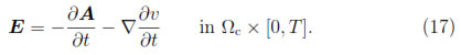
Therefore, the Equation (17) implies that
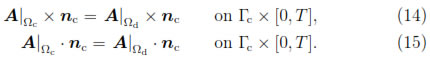
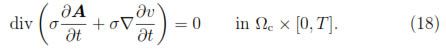
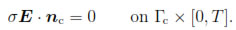
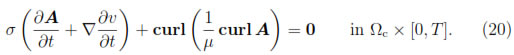
On the other hand, using the Equation (3) together with the Equations (10) and (17), there follows that
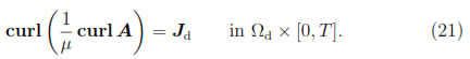
Moreover, from the Equations (5) and (10), we have
The Equations (11)-(15) together with the Equations (18)-(21) will be collected in the potential formulation. Hence, we are led to the following formulation of problem (3)-(9) in terms of the potentials A : Ω x [0, T] 3 and v : Ωc x [0, T] :
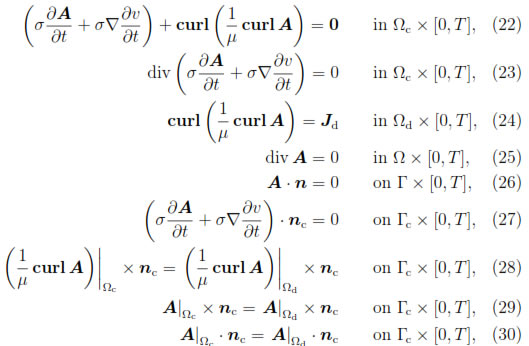
and satisfying
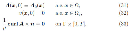
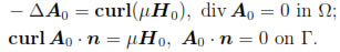
Remark 3.1. Equation (33) is obtained from the Equations (7), (9) and (10), and the Equation (32) is a consequence of (16). Furthermore, the initial condition A0 in (31) must satisfy

and since Ω is a simply connected set, it can be characterized as the unique solution of the boundary value problem (see [23, Theorem I.3.5.]):
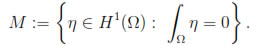
Moreover, A0 can be computed by using a finite element approximation of the following mixed problem [24, Section 4]: find (A0, λ) H(curl; Ω) x M such that
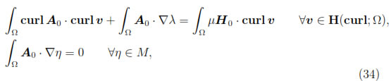
where
In order to prove the well-posedness of this last problem, we can use the well-known Babuska-Brezzi theory for mixed problems (see for instance [25] and the references given there). Furthermore, it follows easily that the Lagrange multiplier λ vanishes identically.
Remark 3.2. The differential constraint (25) is called the Coulomb gauge condition and it is necessary to assure the uniqueness of potential A [13]. The Coulomb gauge condition is not easy to treat at the discrete level, because it is not simple to construct a suitable space of finite elements which are divergence-free. Here we will follow the ideas from [14], by using the addition of a div - div term to our variational formulation (see Section 4 bellow), which is equivalent to add a penalization term in the Ampère law (see, for instance, [13, 14]).
Another possible alternative can be to introduce a Lagrange multiplier (as λ in the Equation (34)) or use an additional scalar magnetic potential. These approaches have been used to impose some differential constraints, which are necessaries for other eddy current formulations, see for instance [4, Chapters 4-5], [5], [7], [10], [15], [26].
4 Variational formulation
The aim of this section is to give a variational formulation of Problem, Equations(22)-(33). To do this, we introduce the following functional spaces:
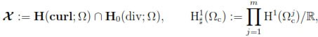
where  are the connected components of Ωc. The spaces X and
  ; (Ωc) are endowed respectively with the norms

and

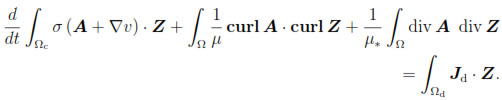
Let Z X. By multiplying the Equations (22) and (24) by Z, integrating in Ωc and Ωd respectively and summing the resulting equations, we deduce that

We notice now that from (22), (24), (28) and Lemma 1 it follows that
Then, by integrating by parts (see (2)) and using (33), we obtain
Hence, from (37) we have
Consequently, if µ* > 0 is a constant (which represents a suitable average of µ in Ω, with µmin≤ µ* ≤ µmax), by using (25), we deduce
for all Z X.
On the other hand, by integrating by parts (1) and using (23) and (27)
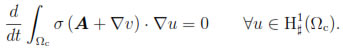
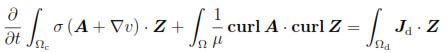
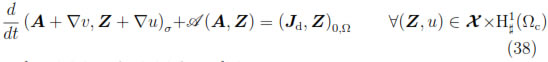
Summing the last two equations, we obtain the following variational formulation of Problem (22)-(33):
Find (A, v) L2(0, T; X x ; (Ωc)) H1(0, T; L2(Ωc)3 x ; (Ωc)) such that
and satisfying the initial condition

where
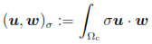
and

Remark 4.1. To our knowledge, the well-posedness of Problem (38)- (39) has not been proved yet. We have tried to apply the theoretical framework for parabolic problems arising from electromagnetism (see Zlámal [27, 28]) and for classical degenerate parabolic problems (see Showalter [29, Chapter III]), without satisfactory results in both cases. However, by adapting the techniques from [27, 28], it is easily seen that Problem (38)-(39) has at most one solution, but this is not the case for the existence result. The main difficulty is that the bilinear form
is not an inner product in L2(Ωc) x ; (Ωc).
Remark 4.2. It is straightforward to verify that a solution of Problem (38)- (39) is actually a solution of the strong form of the problem given by Equations (22)-(33). In particular, we can obtain the gauge condition div A = 0 as follows: for any t [0, T], let ξ H1(Ω) be a weak solution of the compatible Neumann problem Δξ = div A(t) in Ω, ξ/n = 0 on Γ. Hence, by testing (38) with Z :=  ξ and u := -ξΩc+ Ωc-1 Ωc ξ, we obtain
  = 0.
= 0.
Remark 4.3. The idea of using an average µ* to impose the Coulomb gauge condition in the weak formulation is taken from [14]. This is necessary because a finite element approximation based on a weak form, in which the term ∫Ωµ-1div Z div W is present, can be inefficient if the coefficient µ has jumps (see [30, Section 5.7.4]).
5 A fully discrete scheme
In what follows we assume that Ω and Ωc are Lipschitz polyhedra (we recall that Ω is simply-connected). Let {Th}h be a regular family of tetrahedral meshes of Ω such that each element K T his contained either in c or in d. As usual, h stands for the largest diameter of tetrahedra K in Th.
Consider the following finite element spaces:

and

We consider a uniform partition {tn:= nΔt: n = 0, . . . , N} of [0, T] with a step size Δt :=  . For any finite sequence {θn: n = 0, , N}, let
The fully-discrete version of Problem (38)-(39) reads as follows:
Find  such that:

for any (Z, u) Xh x Mh and satisfying

where A0,h Xh is a suitable approximation of A0 to obtain optimal error estimates (see Corollary 6.1 below).
In order to prove that Problem (40)-(41) has a unique solution, we first notice that at each iteration step we need to find  such that

where

Hence, the existence and uniqueness of solution of Problem (40)-(41) follows by combining the Lax-Milgram's Lemma and the following ellipticity result.
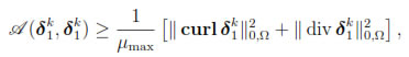
Lemma 2. There exists a constant C > 0 such that

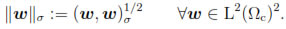
for any Z X and u ; (Ωc).
Proof. First of all, we notice that for Z X, u ; (Ωc) we have
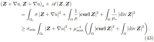
Now, since Ω is a Lipschitz and simply-connected set, there exists a constant C1 > 0 such that (see, for instance, [23, Lemma I.3.6] or [24, Corollary 3.16])

Consequently, from (43), we obtain
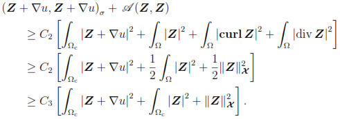
Then by noticing that
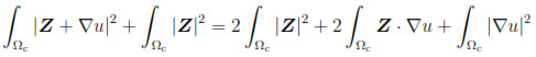
and using the inequality
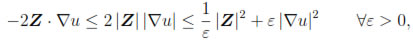
it follows that
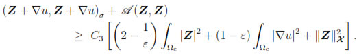
Consequently, by taking 1/2 < ε < 1, we obtain (42).
6 Error estimates
In this section we will prove error estimates for our fully-discrete scheme. To this end, we have to assume that Problem (38)-(39) has a unique solution and consider the elliptic projection operators Ph: X Xh and Qh : ; (Ωc) Mh defined respectively by

and

It is a simple matter to see that Lax-Milgram's Lemma and Lemma 2 imply that Ph and Qh are well defined. Moreover, the well-known Cea's Lemma yields that there exist positive constants C1 and C2, independent of h, such that

and

From now on, let us introduce the following notations:

and

Furthermore, we denote
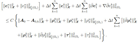
Lemma 3. There exists a positive constant C, independent of h and Δt, such that
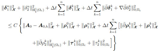
for n = 1, . . . , N.
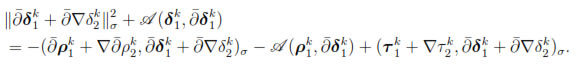
Proof. Let 1 ≤ n ≤ N and 1 ≤ k ≤ n. It is straightforward to show that
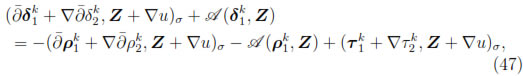
for any (Z, u) Xh x Mh.
Choosing (Z, u) =  in the last identity and using the estimates

and
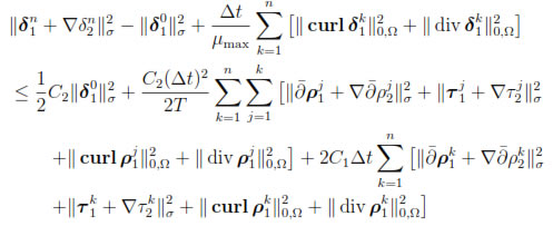
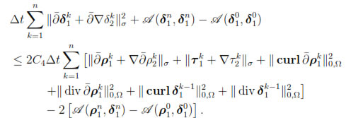
we obtain
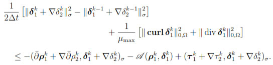
Then, by using the Cauchy-Schwartz inequality in the right hand side, it follows that
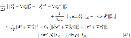
for k = 1, . . . , n. In particular,
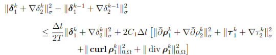
for k = 1, . . . , n. Then, summing over k, we get
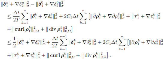
Hence,
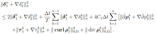
Therefore, the discrete Gronwall's Lemma (see, for instance, [31, Lemma 1.4.2]) leads to
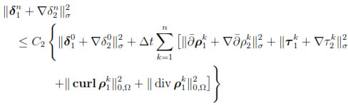
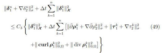
for n = 1, . . . , N. Inserting the last inequality in (48), it follows that
for k = 1, . . . , n. Now, summing over k and recalling that  = 0, we get the estimates
and therefore
Consequently, using (44), we have
for n = 1, . . . , N.
Let us now take (Z, u) =  in (47) to obtain
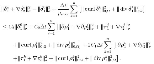
Then,
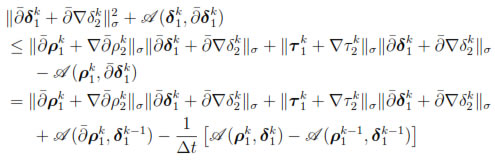
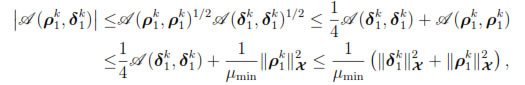
and consequently, using the Cauchy-Schwarz inequality on the right hand side, we deduce that
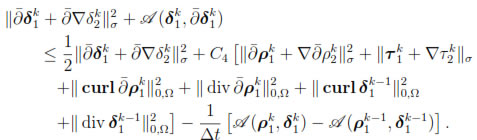
Hence, using the inequality
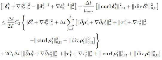
on the left hand side, leads to
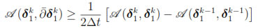
for k = 1, . . . , n. Summing over k, we have
Therefore, by noticing
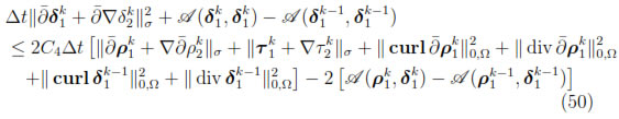
for k = 0, 1, . . . , n, it follows that
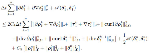
Then, we obtain
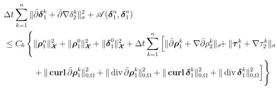
for n = 1, . . . , N.
Combining this last estimate with (49), using Lemma 2 and noticing that

we conclude the desired estimate.
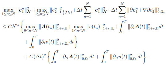
Theorem 6.1. Let  . If
. If

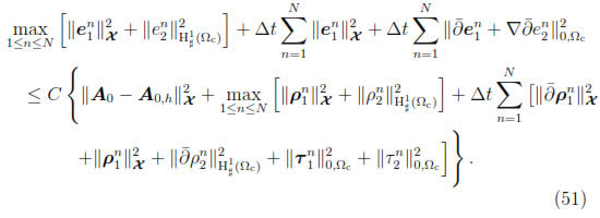
there exists a constant C > 0, independent of h and Δt, such that
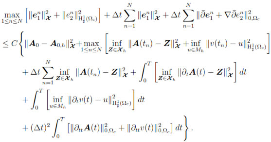
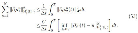
Proof. Since  , from the previous lemma we obtain
Hence
The regularity assumptions on A and v allow us commute the time derivative with Ph and Qh, i.e,

Moreover, if we define  := A(t) - PhA(t) and then from (45) it follows that
and, analogously if := v(t) - Qhv(t), (46) implies
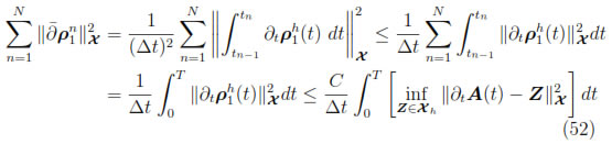
On the other hand, the Cauchy-Schwarz inequality shows that
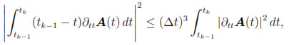
thus, from Taylor's Theorem we have
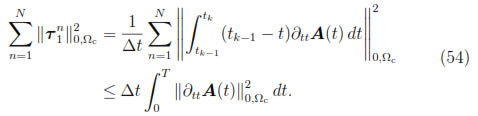
Analogously, we deduce
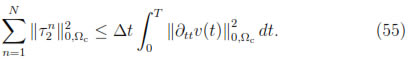
Finally, the result follows from using (52)-(55) and (45)-(46) in (51).
Corollary 6.1. Let and assume that

and

for some 0 < s < 1. If A0,h =Πh(A0), where Πh : X H1+s Xh is the Lagrange interpolant, then there exists a positive constant C, independent of h and Δt, such that
Proof. Let Πh: ; (Ωc) H1+s(Ωc) Mh be the standard scalar finite element Lagrange interpolant. The result follows by using previous theorem, the regularity assumptions on A and v, and the well-known approximation properties of Πh and Πh (see, for instance, [32]).
Remark 6.2. Concerning this convergence result, it has to be noted that the spatial regularity of A (and in particular the regularity of A0) is not ensured if Ω has reentrant corners or edges, namely, if it is a non-convex polyhedron (see [33], [34]). More important, in that case the space H1 H(div; Ω) turns out to be a proper closed subspace of X and hence the nodal finite element approximate solution cannot approach an exact solution A L2(0, T; X) with A  L2(0, T; H1 H(div; Ω)), and convergence in X is lost.
However, the result we have proved here above ensures that the nodal finite element approximation is convergent either if the solution is regular (and this information could be available even for a non-convex polyhedron Ω) or if Ω is a convex polyhedron. Actually, in [17, Section 5] is underlined that if Ω is a convex polyhedron and µH Hpwith 0 < p ≤ 1, the vector potential A (which is characterized by (10)-(12)) belongs to H1+sfor some 0 < s ≤ 1. Let us also note the assumption that Ω is convex is not a severe restriction, as in most real-life applications Ω arises from a somehow arbitrary truncation of the whole space and hence, reentrant corners and edges of Ω can be easily avoided.
A cure for the lack of convergence of nodal finite element approximation for Maxwell equations in the presence of reentrant corners and edges has been proposed by Costabel and Dauge in [35], where they introduce a special weight in the penalization term, thus making it possible to use standard nodal finite elements in a numerically efficient way. Another alternative for the eddy current problem has been reported by Bíró [36]: edge elements are employed for the approximation of the potential A, without requiring that the Coulomb gauge condition be satisfied. However, a complete theory assuring the effectiveness of this last approach, even for the harmonic case, is not available.
To end this section, let us notice that we can approximate at each time tn the physical quantities of interest: the eddy currents σE(tn) in the conductor Ωc and the magnetic induction field µH(tn) in the computational domain Ω. In fact, the identities (17) and (10) suggest the approximations

Moreover, the last corollary allows us to obtain quasi-optimal error estimates for these approximations in some natural discrete L2-norms. In fact, to obtain the error estimate for the first approximation, we notice that
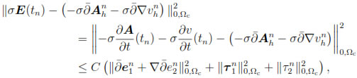
for any n = 1, 2, . . . , N. Therefore, by using (54), (55) and Corollary 6.1, it follows that
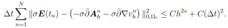
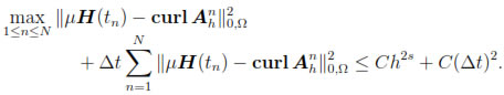
Finally, to get the error estimate for the magnetic induction approximation, we notice that

for n = 1, 2, . . . , N and use Corollary 6.1 to obtain
7 Conclusions
We have proposed a fully-discrete approximation for the so-called ''A, V - A potential formulation'' of a transient eddy current problem in a bounded domain, without topological restrictions on the conductor. The fullydiscrete scheme is obtained by a finite element space discretization of standard nodal finite elements and a time discretization based on a backward-Euler implicit scheme.
We have shown that at each step the fully-discrete scheme solves an elliptic problem and consequently the well-posedness of the discrete problem follows by using the well-known Lax-Milgram's Lemma. Furthermore, under usual regularity assumptions on the solution of the continuous problem, we obtain quasi-optimal error estimates, which allows us to approximate the typical physical variables of interest of the eddy current problem: the eddy currents in the conductor and the magnetic induction in the computational domain.
Acknowledgment
The authors would like to thank the Universidad del Cauca for providing time for this work through research project VRI ID 2665 and anonymous referees for constructive suggestions to the first version of this paper, which allowed us to improve the presentation of this article.
References
[1] A. B. J. Reece and T. W. Preston, Finite Elements Methods in Electrical Power Engineering. New York: Oxford University Press, 2000. [ Links ] 112
[2] A. Bossavit, Computational electromagnetism, ser. Electromagnetism. San Diego, CA: Academic Press Inc., 1998. [ Links ] 112
[3] H. Ammari, A. Buffa, and J.-C. Nédélec, ''A justification of eddy currents model for the Maxwell equations,'' SIAM Journal on Applied Mathematics, vol. 60, no. 5, pp. 1805-1823, 2000. [ Links ] 113
[4] A. Alonso Rodríguez and A. Valli, Eddy current approximation of Maxwell equations, ser. MS&A. Modeling, Simulation and Applications. Springer-Verlag Italia, Milan, 2010, vol. 4. [Online]. Available: http://dx.doi.org/10.1007/978-88-470-1506-7 113, [ Links ] 124
[5] S. Meddahi and V. Selgas, ''An H-based FEM-BEM formulation for a time dependent eddy current problem,'' Applied Numerical Mathematics, vol. 58, no. 8, pp. 1061-1083, 2008. [ Links ] 113, 124
[6] C. Ma, ''The finite element analysis of a decoupled T-Φ scheme for solving eddy- current problems,'' Applied Mathematics and Computation, vol. 205, no. 1, pp. 352-361, 2008. [ Links ] 113
[7] R. Acevedo, S. Meddahi, and R. Rodríguez, ''An E-based mixed formulation for a time-dependent eddy current problem,'' 2009. [ Links ] 113, 124
[8] T. Kang and K. Kim, ''Fully discrete potential-based finite element methods for a transient eddy current problem,'' Computing, vol. 85, no. 4, pp. 339-362, 2009. [ Links ] 113
[9] R. A. Prato Torres, E. P. Stephan, and F. Leydecker, ''A FE/BE coupling for the 3D time-dependent eddy current problem. Part I: a priori error estimates,'' Computing, vol. 88, no. 3-4, pp. 131-154, 2010. [Online]. Available: http://dx.doi.org/10.1007/s00607-010-0089-9 113 [ Links ]
[10] R. Acevedo and S. Meddahi, ''An E-based mixed FEM and BEM coupling for a time-dependent eddy current problem,'' IMA Journal of Numerical Analysis, vol. 31, no. 2, pp. 667-697, 2011. [ Links ] 113, 124
[11] A. Bermúdez, R. López, R. Rodríguez, and P. Salgado, ''Numerical solution of transient eddy current problems with input current intensities as boundary data,'' IMA Journal of Numerical Analysis, vol. 32, pp. 1001-1029, 2012. [ Links ] 113
[12] J. Camaño and R. Rodríguez, ''Analysis of a FEM-BEM model posed on the conducting domain for the time-dependent eddy current problem,'' J. Comput. Appl. Math., vol. 236, no. 13, pp. 3084-3100, 2012. [ Links ] [Online]. Available: http://dx.doi.org/10.1016/j.cam.2012.01.030 113
[13] O. Bíró and K. Preis, ''On the use of the magnetic vector potential in the finite- element analysis of three-dimensional eddy currents,'' Magnetics, IEEE Transactions on, vol. 25, no. 4, pp. 3145-3159, 1989. [ Links ] 113, 120, 121, 124
[14] O. Bíró and A. Valli, ''The Coulomb gauged vector potential formulation for the eddy-current problem in general geometry: wellposedness and numerical approximation,'' Comput. Methods Appl. Mech. Engrg., vol. 196, no. 13-16, pp. 1890-1904, 2007. [ Links ] [Online]. Available: http://dx.doi.org/10.1016/j.cma.2006.10.008 113, 114, 121, 124, 127
[15] A. Bermúdez, R. Rodríguez, and P. Salgado, ''FEM for 3D eddy current problems in bounded domains subject to realistic boundary conditions. An application to metallurgical electrodes,'' Computer Methods in Applied Mechanics and Engineering, vol. 12, no. 1, pp. 67-114, 2005. [ Links ] 113, 124
[16] C. Yongbin, Y. Junyou, Y. Hainian, and T. Renyuan, ''Study on eddy current losses and shielding measures in large power transformers,'' Magnetics, IEEE Transactions on, vol. 30, no. 5, pp. 3068-3071, 1994. [ Links ] 113
[17] R. Acevedo and R. Rodríguez, ''Analysis of the A, V-A-Ψ potential formulation for the eddy current problem in a bounded domain,'' Electron. Trans. Numer. Anal., vol. 26, pp. 270-284, 2007. [ Links ] 114, 140
[18] P. Monk, Finite element methods for Maxwell's equations, ser. Numerical Mathematics and Scientific Computation. New York: Oxford University Press, 2003. [Online]. Available: http://dx.doi.org/10.1093/acprof:oso/9780198508885.001.0001 115, [ Links ] 116, 118
[19] A. Buffa and P. Ciarlet Jr., ''On traces for functional spaces related to Maxwell's equations. I. An integration by parts formula in Lipschitz polyhedra,'' Mathematical Methods in the Applied Sciences, vol. 24, no. 1, pp. 9-30, 2001. [ Links ] 116, 117
[20] A. Buffa and P. Ciarlet Jr., ''On traces for functional spaces related to Maxwell's equations. II. Hodge decompositions on the boundary of Lipschitz polyhedra and applications,'' Mathematical Methods in the Applied Sciences, vol. 24, no. 1, pp. 31-48, 2001. [ Links ] 116
[21] A. Buffa, M. Costabel, and D. Sheen, ''On traces for H(curl,Ω) in Lipschitz domains,'' J. Math. Anal. Appl., vol. 276, no. 2, pp. 845-867, 2002. [ Links ] 116, 117
[22] E. Zeidler, Nonlinear functional analysis and its applications.II/A. New York: Springer-Verlag, 1990. [Online]. Available: http://dx.doi.org/10.1007/978-1-4612-0985-0 119 [ Links ]
[23] V. Girault and P.-A. Raviart, Finite element methods for NavierStokes equations, ser. Springer Series in Computational Mathematics. Berlin:Springer-Verlag, 1986, vol. 5. [Online]. Available: http://dx.doi.org/10.1007/978-3-642-61623-5 121, [ Links ] 124, 129
[24] C. Amrouche, C. Bernardi, M. Dauge, and V. Girault, ''Vector potentials in three-dimensional non-smooth domains,'' Mathematical Methods in the Applied Sciences, vol. 21, no. 9, pp. 823-864, 1998. [ Links ] 124, 129
[25] D. Boffi, F. Brezzi, L. F. Demkowicz, R. G. Durán, R. S. Falk, and M. Fortin, Mixed finite elements, compatibility conditions, and applications, ser. Lecture Notes in Mathematics. Berlin: Springer-Verlag, 2008, vol. 1939. [Online]. Available: http://dx.doi.org/10.1007/978-3-540-78319-0 124
[26] A. Bermúdez, R. Rodríguez, and P. Salgado, ''A finite element method with Lagrange multipliers for low-frequency harmonic Maxwell equations,'' SIAM J. Numer. Anal., vol. 40, no. 5, pp. 1823-1849, 2002. [ Links ] [Online]. Available: http://dx.doi.org/10.1137/S0036142901390780 124
[27] M. Zlámal, ''Finite Element Solution of Quasistationary Nonlinear Magnetic Field,'' Rairo-Analyse numérique, vol. 16, no. 2, pp. 161-191, 1982. [ Links ] 126, 127
[28] M. Zlámal, ''Addendum to the paper 'Finite element solution of quasistationary nonlinear magnetic field','' RAIRO Anal. Numér., vol. 17, no. 4, pp. 407-415, 1983. [ Links ] 126, 127
[29] R. E. Showalter, Monotone operators in Banach space and nonlinear partial differential equations, ser. Mathematical Surveys and Monographs. Providence, RI: American Mathematical Society, 1997, vol. 49. [ Links ] 127
[30] J. Jin, The Finite Element Method in Electromagnetics, 2nd ed. New York: Wiley, 2002. [ Links ] 127
[31] A. Quarteroni and A. Valli, Numerical approximation of partial differential equations, ser. Springer Series in Computational Mathematics. Berlin: Springer- Verlag, 1994, vol. 23. [ Links ] 133
[32] P. G. Ciarlet, The finite element method for elliptic problems, ser. Classics in Applied Mathematics. Philadelphia, PA: Society for Industrial and Applied Mathematics (SIAM), 2002, vol. 40. [Online]. Available: http://dx.doi.org/10.1137/1.9780898719208 140 [ Links ]
[33] M. Costabel and M. Dauge, ''Singularities of electromagnetic fields in polyhedral domains,'' Arch. Ration. Mech. Anal., vol. 151, no. 3, pp. 221-276, 2000. [ Links ] [Online]. Available: http://dx.doi.org/10.1007/s002050050197 140
[34] M. Costabel, M. Dauge, and S. Nicaise, ''Singularities of eddy current problems,'' M2AN Math. Model. Numer. Anal., vol. 37, no. 5, pp. 807-831, 2003. [ Links ] [Online]. Available: http://dx.doi.org/10.1051/m2an:2003056 140
[35] M. Costabel and M. Dauge, ''Weighted regularization of Maxwell equations in polyhedral domains. A rehabilitation of nodal finite elements,'' Numer. Math., vol. 93, no. 2, pp. 239-277, 2002. [ Links ] [Online]. Available: http://dx.doi.org/10.1007/s002110100388 140
[36] O. Bíró, ''Edge element formulations of eddy current problems,'' Comput. Methods Appl. Mech. Engrg., vol. 169, no. 3-4, pp. 391-405, 1999. [ Links ] 140
