ARTÍCULO ORIGINAL

Properties and Applications of Extended Hypergeometric Functions

Propiedades y aplicaciones de Funciones Hipergeométricas Extendida

Daya K. Nagar¹, Raúl Alejandro Morán-Vásquez² and Arjun K. Gupta³

¹ Ph.D. in Science, dayaknagar@yahoo.com, Universidad de Antioquia, Medellín, Colombia.

² Magíster en Matemáticas, alejandromoran77@gmail.com, Universidade de São Paulo, São Paulo, Brasil.

³ Ph.D. in Statistics, gupta@bgsu.edu, Bowling Green State University, Bowling Green, Ohio, USA.

Received: 25-08-2013, Acepted: 16-12-2013

Available online: 30-01-2014

MSC:33C90

Abstract

In this article, we study several properties of extended Gauss hypergeometric and extended confluent hypergeometric functions. We derive several integrals, inequalities and establish relationship between these and other special functions. We also show that these functions occur naturally in statistical distribution theory.

Key words: Beta distribution; extended beta function; extended confluent hypergeometric function; extended Gauss hypergeometric function; gamma distribution; Gauss hypergeometric function.

Resumen

En este artículo estudiamos varias propiedades de las funciones hipergeométrica de Gauss extendida e hipergeométrica confluente extendida. Derivamos varias integrales, desigualdades y establecemos relaciones entre estas y otras funciones especiales. También mostramos que estas funciones ocurren naturalmente en la teoría de distribuciones estadísticas.

Palabras clave: Distribución beta; función beta extendida; función hipergeométrica confluente extendida; función hipergeométrica de Gauss extendida; distribución gamma; función hipergeométrica de Gauss.

1 Introduction

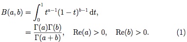
The classical beta function, denoted by B (a, b), is defined (see Luke [1]) by the Euler's integral

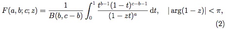
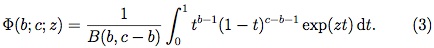
Based on the beta function, the Gauss hypergeometric function, denoted by F(a, b; c; z), and the confluent hypergeometric function, denoted by Φ(b; c; z), for Re(c) > Re(b) > 0, are defined as (see Luke [1]),

and

Using the series expansions of (1 − zt)−^a and exp (zt) in (2) and (3), respectively, the series representations of F(a, b; c; z) and Φ(b; c; z), for Re(c) > Re(b) > 0, are obtained as

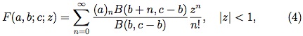
and

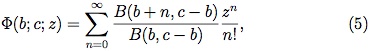
respectively.

In 1997, Chaudhry et al. [2] extended the classical beta function to the whole complex plane by introducing in the integrand of (1) the exponential factor exp [− σ ⁄ t (1 − t)], with Re(σ) > 0. Thus, the extended beta function is defined as

If we take σ = 0 in (6), then for Re(a) > 0 and Re(b) > 0 we have B(a, b; 0) = B(a, b). Further, replacing t by 1 − t in (6), one can see that B(a, b; σ) = B(b, a; σ). The rationale and justification for introducing this function are given in Chaudhry et al. [2] where several properties and a statistical application have also been studied. Miller [3] further studied this function and has given several additional results.

In 2004, Chaudhry et al. [4] gave definitions of the extended Gauss hypergeometric function and the extended confluent hypergeometric function, denoted by F_σ (a, b; c; z) and Φ_σ (b; c; z), respectively. These definitions were developed by considering the extended beta function (6) instead of beta function (1) that appear in the general term of the series (4) and (5). Thus, for Re(c) > Re(b) > 0, F_σ (a, b; c; z) and Φ_σ (b; c; z) are defined by

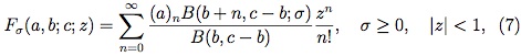
and

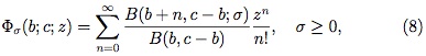
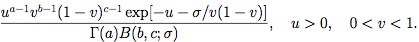
respectively. Further, using the integral representation of the extended beta function (6) in (7) and (8), Chaudhry et al. [4] obtained integral representations, for σ ≥ 0 and Re(c) > Re(b) > 0, of the extended Gauss hypergeometric function (EGHF) and the extended confluent hypergeometric function (ECHF) as

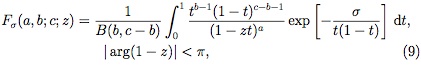
and

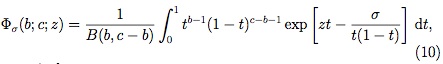
respectively.

For σ = 0 in (9), we have F₀ (a, b; c; z) = F(a, b; c; z), that is, the classical Gauss hypergeometric function is a special case of the extended Gauss hypergeometric function. Likewise, taking σ = 0 in (10) yields Φ₀ (b; c; z) = Φ(b; c; z), which means that the classical confluent hypergeometric function is a special case of the extended confluent hypergeometric function. Chaudhry et al. [4] and Miller [3] found that extended forms of beta and hypergeometric functions are related to the beta, Bessel and Whittaker functions, and also gave several alternative integral representations.

In this article, we give several interesting results on extended beta, extended Gauss hypergeometric and extended confluent hypergeometric functions and show that they occur in a natural way in statistical distribution theory.

This paper is divided into five sections. Section 2 deals with some well known definitions and results on special functions . In Section 3, several properties of the extended beta, the extended Gauss hypergeometric and the extended confluent hypergeometric functions have been studied. Section 4 deals with the integrals involving EGHF and ECHF. Finally, applications of the extended Gauss hypergeometric and the extended confluent hypergeometric functions are demonstrated in Section 5.

2 Some Known Definitions and Results

An integral representation of the type 2 modified Bessel function (Gradshteyn and Ryzhik [5, Eq. 3.471.9]) is given by

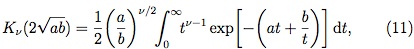
where Re(a) > 0 and Re(b) > 0.

If we make the transformation t = (1 + u)⁻¹u in (2) and (3) with the Jacobian J(t u) = (1 + u)⁻², we obtain alternative integral representations for F(a, b; c; z) and Φ(b; c; z) as

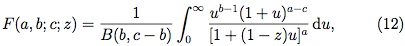
and

respectively.

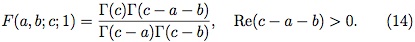
Putting z = 1 in (2) and evaluating the resulting integral using (1), one obtains

In the remainder of this section we give several properties of extended beta, extended Gauss hypergeometric, and extended confluent hypergeometric functions, most of them have been derived by Chaudhry et al. [2],[4].

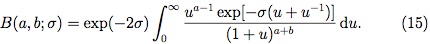
Using the transformation t = (1 + u)⁻¹u in (6), with the Jacobian J(t u) = (1 + u)⁻², we arrive at

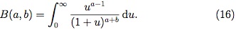
For σ = 0 with Re(a) > 0 and Re(b) > 0, the above expression gives the well-known integral representation of B(a, b) as

If we take b = −a in (15) and compare the resulting expression with (11) we obtain an interesting relationship between the extended beta function and the type 2 modified Bessel function as

If we consider z = 1 in (9) and compare the resulting expression with the representation (6), we find that the extended beta function and EGHF are related by the expression

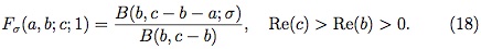
Further, substituting c = a in (18) and using (17), we obtain, for σ > 0,

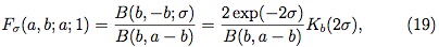
where Re(a) > Re(b) > 0.

Note that (19) can also be obtained by taking z = 1 and a = c in (20), and then using the integral representation (11).

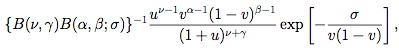
In the integral representation of EGHF and ECHF given in (9) and (10), respectively, substituting t = (1 + u)⁻¹u, with the Jacobian J(t u)= (1 + u)⁻², alternative integral representations are obtained as

and

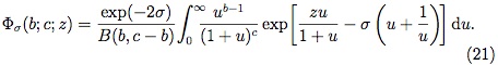
If we take σ = 0 in (20) and (21), we arrive at the representations (12) and (13) of the classical Gauss hypergeometric function and the classical confluent hypergeometric function, respectively.

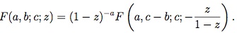
For | arg(1 − z) | < 1, the transformation formula is given by

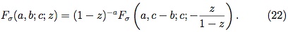
It is noteworthy that σ = 0 in (22) gives the well-known transformation formula

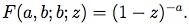
Also, putting c = b in the above expression, one obtains

In the integral representation of the ECHF (10) consider the substitution 1 − u = t, whose Jacobian is given by J(t u) = 1, to obtain

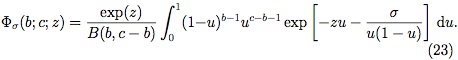
By evaluating the integral in (23) using (10), Kummer's relation for extended confluent hypergeometric function is derived as

For σ = 0, the expression (24) reduces to the well known Kummer's first formula for the classical confluent hypergeometric function.

3 Properties of the EGHF and ECHF

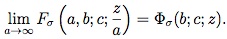
This section gives several properties of the the EGHF and ECHF. Writing F_σ (a, b; c; z ⁄a) in terms of integral representation using (9) and taking a ∞, we obtain

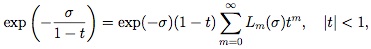
Replacing exp(− σ ⁄ t) and exp[− σ ⁄ (1 − t)] by their respective series expansions involving Laguerre polynomials (n = 0, 1, 2...) given in Miller [3, Eq. 3.4a, 3.4b], namely,

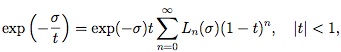
and

in (9) and (10), and integrating with respect to t using (2) and (3), EGHF and ECHF can also be expressed as

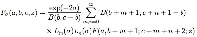
and

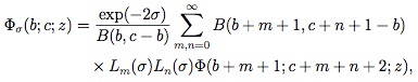
respectively.

Theorem 3.1. If z is such that z < 1, σ > 0 and c > b > 0, then

Proof. It follows that for u > 0 and σ > 0, σ ≥ 0 implies that σ(u + u⁻¹) ≥ 2 σ and exp[−σ (u + u⁻¹)] ≤ exp(−2 σ). Now, using this inequality in the representation given in (20), we get

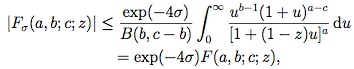
where the last line has been obtained by using (12). Further, the inequality ln v ≤ v − 1, v > 0, for v = 4 σ, yields

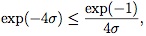
which gives the second part of the inequality.

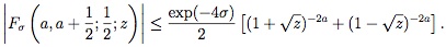
Using special cases of the Gauss hypergeometric function in (25), several inequalities for EGHF can be obtained. For example, application of

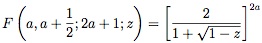
and

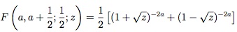
yield

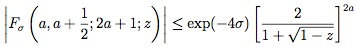
and

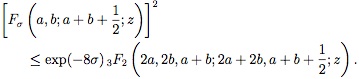
Further, using the Clausen's identity

in (25), one gets

If we put z = 1 in (25), and then use (18) and (14) in the resulting expression, we obtain

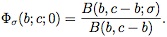
where d = c−a−b > 0. If we replace z = 0 in (10) and compare the resulting expression with (6), we see that the ECHF and the extended beta function have the relationship

Theorem 3.2. If α and β are two scalars such that β − α > 0, then

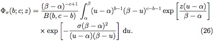
Proof. Using the transformation t = (u − α) ⁄ (β − α) with the Jacobian (β − α)⁻¹in the representation (10), we obtain the result.

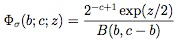
If we consider β = 1 and α = −1 in (26), we have another integral representation of extended confluent hypergeometric function as

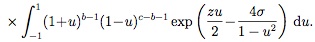
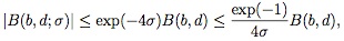
Theorem 3.3. If σ > 0 and c > b > 0, then

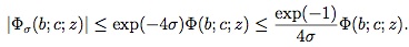
Proof. Similar to the proof of Theorem 3.1.

4 Integrals involving EGHF and ECHF

In this section we evaluate some integrals that are related to EGHF and ECHF.

Theorem 4.1. If σ ≥ 0, α > β > 0, Re(c) > Re(b) > 0 and Re(a) > 0, then

Proof. Using the integral representation (10) and changing the order of integration, we have

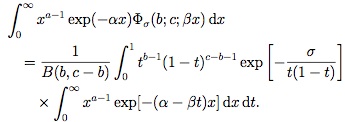
Now, integrating with respect to x using Euler's gamma integral and then t using the representation (9), we get the desired result.

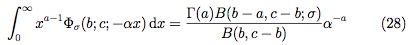
Corollary 4.1. If σ > 0, α > 0, Re(c) > Re(b) > 0 and Re(a) > 0, then

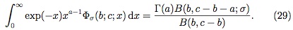
and

Proof. Application of Kummer's relation (24) yields

Evaluating the above integral by applying (27) and then using the relation (18), we get (28). To prove (29) just take α = β = 1 in (27) and use (18).

Corollary 4.2. If σ > 0 and Re(c) > Re(b) > 0, then

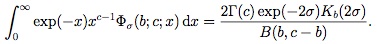
Proof. Just take a = c in (29), and then use (17).

Theorem 4.2. For σ ≥ 0, α < 1, Re(a) > Re(d) > 0 and Re(c) > Re(b) > 0, we have

Proof. Using (9) and changing the order of integration

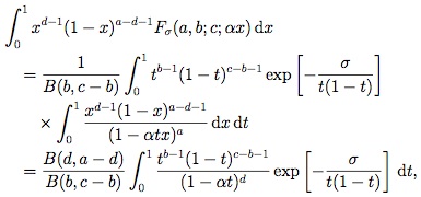
where the integral involving x has been evaluated using (2). Finally, using the representation (9), we arrive at the desired result.

Corollary 4.3. For σ > 0 and Re(a) > Re(c) > Re(b) > 0, we have

Proof. Just take α = 1 and c = d in (30), and then use (19).

Theorem 4.3. For σ > 0, Re(c) > Re(b) > 0 and Re(a) > Re(d) > 0, we have

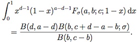
Proof. Using (30), one gets

Now, replacing d and a − d by a − d and d, respectively, in the above expression, one gets

Finally, substituting for F_σ (a − d, b; c; 1) from (18), we get the desired result.

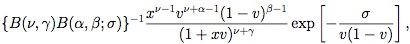
Theorem 4.4. If σ > 0, α > 0, Re(a) > Re(d) > 0 and Re(c) > Re(b) > 0, then

Proof. Replacing F_σ (a, b; c; −αx) by its integral representation (9) and changing the order of integration, we get

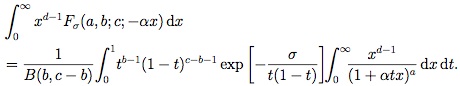
Now, we integrate x using (16) and then t using (6) to obtain the result.

Corollary 4.4. If σ > 0, α > 0 and Re(a) > Re(c) > Re(b) > 0, then

Proof. Just take c = d in (31) and use the relation (17).

5 Statistical Distributions

In this section, we define the extended Gauss hypergeometric function and the extended confluent hypergeometric function distributions. We study several properties of these new distributions and their relationships with other known distributions. We also show that these distributions occur naturally as the distribution of the quotient U/V , where U and V are independent, U has a gamma or beta type 2 distribution and the random variable V has an extended beta type 1 distribution. In the end, we derive results on products and quotients of independent random variables.

First, we define the gamma, beta type 1 and beta type 2 distributions. These definitions can be found in Johnson, Kotz and Balakrishnan [6], and Gupta and Nagar [7].

A random variable X is said to have a gamma distribution with parameters θ (> 0),κ (> 0), denoted by X Ga(κ, θ), if its probability density function (pdf) is given by

Note that for θ = 1, the above distribution reduces to a standard gamma distribution and in this case we write X Ga(κ).

A random variable X is said to have a beta type 1 distribution with parameters (a, b), a > 0, b > 0, denoted as X B1(a, b), if its pdf is given by

where B(a, b) is the beta function.

A random variable X is said to have a beta type 2 distribution with parameters (a, b), denoted as X B2(a, b), a > 0, b > 0, if its pdf is given by

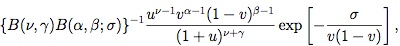
A random variable X is said to have an extended beta (type 1) distribution with parameters α, β and λ, denoted by X EB1(α, β; λ), if its pdf is given by (Chaudhry et al. [2]),

where B(α, β; λ) is the extended beta function defined by (6), λ > 0, and −∞ < α, β < ∞.

For λ = 0 with α > 0 and β > 0, the density (34) reduces to a beta type 1 density.

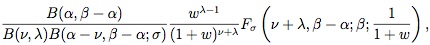
Definition 5.1. A random variable X is said to have an extended Gauss hypergeometric function distribution with parameters ν, α, β, γ and σ, denoted by X EGH(ν, α, β, γ; σ), if its pdf is given by

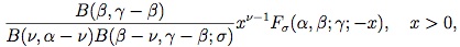
where α > ν > 0, γ > β > 0 if σ > 0 and α > ν > 0, γ > β > ν > 0 if σ = 0.

The following theorem derives the extended Gauss hypergeometric function distribution as the distribution of the ratio of two independent random variables distributed as beta type 2 and extended beta type 1.

Theorem 5.1. Suppose that the random variables U and V are independent, U B2(ν, γ) and V EB1(α, β; σ). Then U/V EGH(ν, ν + γ, ν + α, ν + α + β; σ).

Proof. As U and V are independent, by (33) and (34), the joint density of U and V is given by

where u > 0 and 0 < u < 1. Using the transformation X = U/V , with the Jacobian J(u x) = u, we obtain the joint density of V and X as

where 0 < u < 1 and x > 0. Now, integration of the above expression with respect to u using (9) yields the desired result.

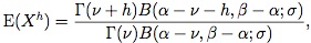
If X EGH(ν, α, β, γ; σ), then

Now, evaluation of the above integral by using (31) yields

where −ν < Re(h) < α − ν if σ > 0, and −ν < Re(h) < α − ν and Re(h) < β − ν if σ = 0.

Next, we define and study the extended confluent hypergeometric function distribution.

Definition 5.2. A random variable X is said to have an extended confluent hypergeometric function distribution with parameters (ν, α, β, σ), denoted by X ECH(ν, α, β; σ), if its pdf is given by

where ν > 0, β > α > 0 if σ > 0 and β > α > ν > 0 if σ = 0.

The extended confluent hypergeometric function distribution can be derived as the distribution of the quotient of independent gamma and extended beta type 1 variables as given in the following theorem.

Theorem 5.2. If U Ga(a) and V EB1(b, c; σ) are independent, then X = U/V ECH(a, a + b, a + b + c; σ).

Proof. As U and V are independent, from (32) and (34), the joint density of U and V is given by

Making the transformation X = U/V , with the Jacobian J(u x) = ν, we find the joint density of V and X as

Now, the density of X is obtained by integrating the above expression with respect to v using the integral representation (10).

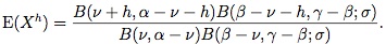
By using (28), the expected value of X ^h, when X ECH(ν, α, β; σ), is derived as

where Re(ν + h) > 0 if σ > 0 and β > α > Re(ν + h) > 0 if σ = 0.

In the remainder of this section we derive results on products and quotients of independent random variables. The derivation and final result in each case involves extended forms of beta, confluent hypergeometric, Gauss hypergeometric or generalized hypergeometric functions showing ample applications of these functions and further advancing statistical distribution theory.

Theorem 5.3. Suppose that the random variables X and Y are independent, X Ga(λ) and Y ECH(ν, α, β; σ). Then, the pdf of R = Y/(Y + X) is given by

where 0 < r < 1.

Proof. Since X and Y are independent, from (32) and (35), we write the joint density of X and Y as

where x > 0 and y > 0. Now, making the transformation S = Y +X and R = Y/(Y + X) with the Jacobian J(x, y r, s) = s and using (24), we obtain the joint density of S and R as

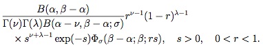
Clearly, R and S are not independent. Integrating the previous expression with respect to s by using (27) the density of R is obtained.

Corollary 5.1. The density of W = X/Y is given by

where w > 0.

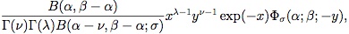
Theorem 5.4. Suppose that the random variables U and V are independent, U B2(ν, γ) and V EB1(α, β; σ). Then Y = UV has the density

Proof. As U and V are independent, from (33) and (34), the joint density of U and V is given by

where u > 0 and 0 < u < 1. Using the transformation Y = UV , with the Jacobian J(u y) = 1/v, we obtain the joint density of V and Y as

where 0 < u < 1 and y > 0. The marginal density of Y is obtained by integrating the above expression with respect to v using (9).

Corollary 5.2. Suppose that the random variables U and V are independent, U B2(ν, γ) and V B1(α, β). Then Y = UV has the density

The above corollary has also been derived in Nagar and Zarrazola [8] and Morán-Vásquez and Nagar [9].

6 Conclusion

We have given several interesting properties of extended beta, extended Gauss hypergeometric and extended confluent hypergeometric functions. We have also evaluated a number of integrals involving these function. Finally, we have shown that these functions occur in a natural way in statistical distribution theory.

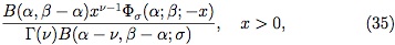
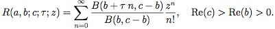
In a series of papers Castillo-Pérez and his co-authors [10],[11],[12],[13] have studied a generalization of the Gauss hypergeometric function defined by

Replacing B(b + τ n,c − b) by B(b + τ n,c − b; σ), an extended form of the above function can be defined as

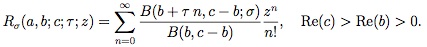
The function defined above is a generalization of the extended Gauss hypergeometric function and will be considered for further research.

Acknowledgements

The research work of DKN was supported by the Sistema Universitario de Investigación, Universidad de Antioquia under the project no. IN10182CE.

References

[1] Y. L. Luke, The special functions and their approximations, Vol. I, ser. Mathematics in Science and Engineering, Vol. 53. New York: Academic Press, 1969.         [ Links ] 12

[2] M. A. Chaudhry, A. Qadir, M. Rafique, and S. M. Zubair, ''Extension of Euler's beta function,'' J. Comput. Appl. Math., vol. 78, no. 1, pp. 19-32, 1997.         [ Links ] [Online]. Available: http://dx.doi.org/10.1016/S0377-0427(96)00102-1 13, 15, 25

[3] A. R. Miller, ''Remarks on a generalized beta function,'' J. Comput. Appl. Math., vol. 100, no. 1, pp. 23-32, 1998.         [ Links ] [Online]. Available: http://dx.doi.org/10.1016/S0377-0427(98)00121-6 13, 14, 18

[4] M. A. Chaudhry, A. Qadir, H. M. Srivastava, and R. B. Paris, ''Extended hypergeometric and confluent hypergeometric functions,'' Appl. Math. Comput., vol. 159, no. 2, pp. 589-602, 2004.         [ Links ] [Online]. Available: http://dx.doi.org/10.1016/j.amc.2003.09.017 13, 14, 15

[5] I. S. Gradshteyn and I. M. Ryzhik, Table of integrals, series, and products, 7th ed. Elsevier/Academic Press, Amsterdam, 2007, translated from the Russian, Translation edited and with a preface by Alan Jeffrey and Daniel Zwillinger, With one CD-ROM (Windows, Macintosh and UNIX).         [ Links ] 15

[6] N. L. Johnson, S. Kotz, and N. Balakrishnan, Continuous univariate distributions. Vol. 2, 2nd ed., ser. Wiley Series in Probability and Mathematical Statistics: Applied Probability and Statistics. New York: John Wiley & Sons Inc., 1995, a Wiley-Interscience Publication.         [ Links ] 24

[7] A. K. Gupta and D. K. Nagar, Matrix variate distributions, ser. Chapman & Hall/CRC Monographs and Surveys in Pure and Applied Mathematics. Chapman & Hall/CRC, Boca Raton, FL, 2000, vol. 104.         [ Links ] 24

[8] D. K. Nagar and E. Zarrazola, ''Distributions of the product and the quotient of independent Kummer-beta variables,'' Sci. Math. Jpn., vol. 61, no. 1, pp. 109-117, 2005.         [ Links ] [Online]. Available: http://www.jams.or.jp/scm/contents/e-2004-1/2004-4.pdf 29

[9] R. A. Morán-Vásquez and D. K. Nagar, ''Product and quotients of independent Kummer-gamma variables,'' Far East J. Theor. Stat., vol. 27, no. 1, pp. 41-55, 2009.         [ Links ] 29

[10] J. A. Castillo Pérez and C. Jiménez Ruiz, ''Algunas representaciones simples de la función hipergeométrica generalizada 2^r1(a, b; c; τ ; x),'' Ingeniería y Ciencia, vol. 2, no. 4, pp. 75-94, 2006.         [ Links ] [Online]. Available: http://publicaciones.eafit.edu.co/index.php/ingciencia/article/view/464 30

[11] J. A. Castillo Pérez, ''Algunas integrales impropias con límites de integración infinitos que involucran a la generalización τ de la función hipergeométrica de gauss,'' Ingeniería y Ciencia, vol. 3, no. 5, pp. 67-85, 2007.         [ Links ] [Online]. Available: http://publicaciones.eafit.edu.co/index.php/ingciencia/article/view/456 30

[12] J. A. Castillo Pérez, ''Algunas integrales que involucran a la función hipergeométrica generalizada,'' Ingeniería y Ciencia, vol. 4, no. 7, pp. 7-22, 2008.         [ Links ] [Online]. Available: http://publicaciones.eafit.edu.co/index.php/ingciencia/article/view/224 30

[13] J. A. Castillo Pérez and L. Galué, ''Algunas integrales indefinidas que contienen a la función hipergeométrica generalizada,'' Ingeniería y Ciencia, vol. 5, no. 9, pp. 45-54, 2009.         [ Links ] [Online]. Available: http://publicaciones.eafit.edu.co/index.php/ingciencia/article/view/467 30