


Services on Demand
Journal
Article
 English (pdf)
 Article in xml format
 Article references
 Send this article by e-mail
Indicators
-
 Cited by SciELO
 -
 Access statistics
Related links
-
 Cited by Google
 -
 Similars in
SciELO
Similars in
SciELO -
 Similars in Google
Share

 Permalink
Ingeniería y Ciencia
Print version ISSN 1794-9165
ing.cienc. vol.11 no.21 Medellín Jan./June 2015
https://doi.org/10.17230/ingciencia.11.21.1
ARTÍCULO ORIGINAL
doi:10.17230/ingciencia.11.21.1
Least Change Secant Update Methods for Nonlinear Complementarity Problem
Métodos secantes de cambio mínimo para el problema de complementariedad no lineal
Favián Arenas A.1, Héctor J. Martínez2 and Rosana Pérez M.3
1 Universidad del Cauca, Popayán, Colombia, farenas@unicauca.edu.co.edu.co.
2 Universidad del Valle, Cali, Colombia, hector.martinez@correounivalle.edu.co.
3 Universidad del Cauca, Popayán, Colombia, rosana@unicauca.edu.co.
Received: 16-12-2013 | Acepted: 20-05-2014 | Online: 30-01-2015
MSC: 90C30, 90C33, 90C53
Abstract
In this work, we introduce a family of Least Change Secant Update Methods for solving Nonlinear Complementarity Problems based on its reformulation as a nonsmooth system using the one-parametric class of nonlinear complementarity functions introduced by Kanzow and Kleinmichel. We prove local and superlinear convergence for the algorithms. Some numerical experiments show a good performance of this algorithm.
Key words: nonsmooth systems; nonlinear complementarity problems; generalized Jacobian; quasi-Newton methods; least change secant update methods; local convergence; superlinear convergence
Resumen
En este trabajo generamos una familia de métodos secante de cambio mínimo para resolver Problemas de Complementariedad no Lineal vía su reformulación como un sistema de ecuaciones no lineales no diferenciable usando una clase de funciones de complementariedad propuesta por Kanzow and Kleinmichel. Bajo ciertas hipótesis demostramos que esta familia proporciona algoritmos local y superlinealmente convergentes. Experimentos numéricos preliminares demuestran un buen desempeño de los algoritmos propuestos.
Palabras clave: sistemas no diferenciables; complementariedad no lineal; métodos cuasi-Newton
1 Introduction
Let F: n → n,F(x)=(F1(x),…,Fn(x)) be a continuously differentiable mapping. The Nonlinear Complementarity Problem, NCP for short, consists of finding a vector x
  n such that,
Here, y ≥ 0 for y n means yi ≥ 0 for all i=1,…,n. The third condition in (1) requires that the vectors x and F(x) are orthogonal; for this reason, it is called complementarity condition.
The NCP arises in many applications such as Friction Mechanical Contact problems [1], Structural Mechanics Design problems, Lubrication Elasto-hydrodynamic problems [2], Traffic Equilibrium problems [3], as well as problems related to Economic Equilibrium Models [4]. The importance of NCP in the areas of Physics, Engineering and Economics is due to the fact that the concept of complementarity is synonymous with the notion of system in equilibrium. In recent years, various techniques have been studied to solve the NCP, one of which is to reformulate it as a nonsmooth system of nonlinear equations by using special functions called complementarity functions [5]. A function φ:2→ such that

is called a complementarity function.
Geometrically, the equivalence (2) means that the trace of the function φ obtained by the intersection with the xy plane is the curve formed by the positive semiaxes x and y, which is not differentiable at (0,0). This lack of smoothness on the curve imply the nondifferentiability of the function φ.
In order to reformulate the NCP as a system of nonlinear equations, it is necessary to consider a complementarity function φ and to define Φ:n→ n by
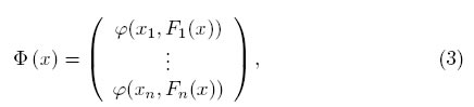
then it follows from lack of smoothness of φ that the nonlinear system of equations
is nonsmooth. From the definition of a complementarity function (2) it follows that a vector x* solves the system (4), if and only if, x* solves the NCP. Different algorithms have been proposed for solving the reformulation of the NCP by a nonsmooth system of nonlinear equations (4) like nonsmooth Newton methods [6], nonsmooth quasi-Newton methods [7],[8],[9], among others [10], [11],[12],[13].
There are many complementarity functions, but the most used has been the minimum function [14] and the Fischer-Burmeister function[15], defined respectively by

The minimum function is nonsmooth at the points of the form (a,a), while the Fischer-Burmeister function is not nonsmooth at (0,0). In 1998, Kanzow and Kleinmichel [15] introduced an one-parametric class of complementarity functions φλ defined by

where λ (0,4) and which we will refer to throughout this work as Kanzow function. This function is nonsmooth at (0,0). For any other vector in 2, the gradient vector of φλ is defined by
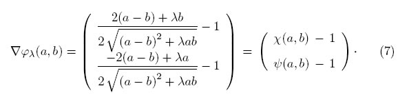
In [16], the author makes a carefully analysis of this function and deduces some important bounds that we will use later. Moreover, In the special case λ = 2, the function φλ reduces to theFischer-Burmeister function, whereas in the limiting case λ→ 0, the function φλ becomes a multiple of the minimum function. In what follows, we denote by Φλ the function defined in (3) and obtained by the complementarity function φλ.
In this work, we propose a nonsmooth quasi Newton method for solving the NCP using the system Φλ(x)=0; for this method, we prove local convergence. Moreover, we introduce a family of least change secant update for solving the NCP based on the nonsmooth system of equations Φλ(x)=0 and, for these family, we prove local and superlinear convergence under suitable assumptions.
We organize this paper as follows. In Section 2, we reformulate the NCP as a nonsmooth system of equations using the Φλ function and we characterize a subset of the generalized Jacobian of Φλ in x. In the first part of Section 3, we propose a new algorithm quasi-Newton for solving the nonsmooth system of nonlinear equations Φλ (x)=0 and, for this method, we develop the local convergence theory. In the second part, we introduce a family of least change secant update methods following the theory developed in [17] for this type of methods. We prove, under suitable assumptions, local and superlinear convergence. In Section 4, we analyze numerically, the local performance of the algorithms introduced in the last section, for which we use 8 test problems proposed in [14],[18]. Four of this are applications problems to Economic Equilibrium and Game Theory. Finally, Section 5 contains some remarks on what we have done in this paper and present possibilities for future works.
2 Reformulation of NCP using the Kanzow function
In this section, we reformulate the NCP as a nonsmooth system of equations and from the definition of the generalized Jacobian given in [19], we construct a subset of matrices of the generalized Jacobian of Φλ at x. Then we show that this subset at a solution of the system Φλ(x) = 0 is a compact set.
Our reformulation of NCP as a system of equations is based on the Kanzow complementarity function φλ defined by (6) and the Φλ function defined in the last section. Exploiting (2) it is readily seen that the NCP is equivalent to the following system of nonsmooth equations
The most popular method for solving a differentiable system of nonlinear equations G(x)=0 is Newton's method [8], which require calculating, at each iteration, the Jacobian matrix of G. There are situations where the derivatives of G are not available, or are difficult to calculate. For this cases, a less expensive alternative and widely used for solving G(x)=0 are the quasi-Newton methods [8] which use, at each iteration, a matrix approximation to the Jacobian matrix. Among the latter are the so-called least change secant update methods [10] , which form a family characterized by the fact that, at each iteration, the Jacobian approximation satisfies a secant equation [10] with a minimum variation property relative to some matrix norm. The price of using an approximation to the Jacobian Matrix is reflected in the decrease of the speed of convergence of the respective quasi-Newton method.
When a function is not differentiable as in the case of the function Φλ, the term ''Jacobian matrix'' does not make sense. Fortunately, Frank H. Clarke introduced the concept of Generalized Jacobian that extends the matrix Jacobian concept for some non-differentiable functions [19]. Let F:n→ n be a locally Lipschitzian function. The Generalized Jacobian of F at x is the set given by

Since the Kanzow function φλ is locally Lipschitz continuous [16], so is the Φλ function. Thus, the Generalized Jacobian of Φλ(x) exists. In order to build matrices in this set, we consider a sequence of vectors in n, {yk}, which converges to x and such that Φ'λ (yk) exists, then we show that  exists. To classify the indices of the components of x, we define the set

The sequence1 that we will use is

where {εk} is a sequence of positive numbers such that  εk=0 and the vector z is chosen such that zi ≠ 0 where i β . Obviously yk converges to x when k→ ∞. To analyze the differentiability of Φλ in yk, we consider two cases. If i
  β then xi ≠ 0 or Fi(x) ≠ 0 , by the continuity of Fi, we can assume εk so small that
  ≠ 0 or Fi(x) ≠ 0, for which Φλ is differentiable at yk. If i β, the zi ≠ 0; therefore, ≠ 0 , which is sufficient for Φλ to be differentiable at yk.
By differentiability of Φλ at yk, the Jacobian matrix of Φλ at yk, exist and its i th row is given by

with χ and ψ defined by (7) and {e1,…,en} is the canonical basis of n.
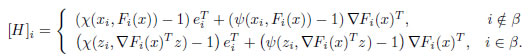
For calculating the Φ'λ (yk), we consider two cases: If i β, by continuity of i th row of Φ'λ ( yk) we have ∇φ λ (y,Fi(yk))T is [H]i where [H]i = ( χ(xi,Fi(x)) −1 )  + (ψ(xi,Fi(x)) −1 ) ∇Fi(x)T. If i β, from (11), we have
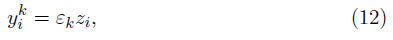
further, by the Taylor's theorem,

where ζk → x when k→ ∞. Substituting (12) and (13) in the i th row of Φ'λ (yk), i β, we obtain
with[H]i = ( χ(zi ,∇Fi(x)Tz) −1) + ( ψ(zi ,∇Fi(x)Tz) −1 )∇Fi(x)T. Then, for all i=1,…,n, the limit when k→ ∞ of each row of Φλ′(yk) exist. Therefore,
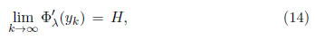
where
Because there is an uncountable of ways of choosing the vector z, we have an uncountable set of matrices H in ∂Φλ(x) which can be calculated by the above procedure.
Now, we consider the particular case where x* is a solution of Φλ (x) = 0. If there is any index i such that xi=Fi(x*)=0, then x* is called a degenerate solution. We will denote the matrices (14) in x* by H*(z). The set of these matrices we will call  . Clearly, for each z n, there is a matrix H*(z). Thus, is an infinite set and further it is a compact set. To verify the compactness, it is sufficient to demonstrate that it is closed, since ⊆ ∂Φ(x*), which is compact [19], [16].
3 Algorithm and convergence theory
In the first part of this section, we propose a new quasi-Newton algorithm for solving the system Φλ (x)=0 and we develop the local convergence theory for this method. In the second part, we develop a family of least change secant update methods, following [17]. For these family, we prove local and superlinear convergence under suitable assumptions. The following algorithm is the basic quasi-Newton algorithm applied to Φλ (x)=0.
Algorithm 1 Given x0 an initial approximation to the solution of the problem and λ (0,4), compute xk+1=xk−Bk−1Φλ (xk), for k=1,2,…, where
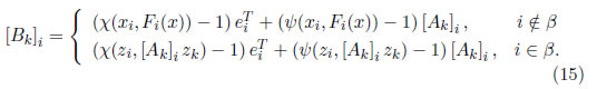
Here {e1, …,en } is a canonical basis of n, the matrix Ak is an approximation of the Jacobian matrix of F at xk (to see Section 6) and zk n is such that  ≠ 0, if
  = Fi(xk) = 0.
Under the following assumptions, we will prove that the sequence generated by the basic quasi-Newton Algorithm 1is well define and converges linearly to a solution of Φλ (x)=0.
3.1 Local assumptions
H1. There is x* n such that Φλ (x*) = 0.
H2. The jacobian matrix of F is Lipschitz continuous (with constant γ) in a neighborhood of x* n.
H3. The matrices of the set Z* are nonsingular. From assumption H3 and by the compactness of , we have that there is a constant μ such that for all H*(z) ,
3.2 A local convergence theory
The following two Lemmas prepare the ''Theorem of the two neighborhoods''.
Lemma 1 Let F:n→ n, F C1, such that its Jacobian matrix verifies H2, the matrices H and B defined by (14) and (15), respectively, and given positive constants ϵ and δ. Then, for each x  (x* ; ϵ) and A (F′(x*) ;δ), there exists a positive constant θ such that
 z∞+n ηz∞∇Fj(x*)∞+√2 n + n andω = nγ (√2+ 1 ).
 See proof in [16].
Lemma 2 Let r (0,1) and B the matrix defined by (15). There exist positive constants ϵ0 and δ0 such that,

 defined by
is well defined, and satisfies

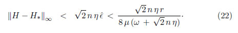
Let r (0,1), > 0 and δ0 > 0 such as
  and δ0<
  , where ω is the constant (17), η is the Lipschitz constant of ∇φλ given by [16] and τ and μ are defined by Lemma 3.1. We take x (x* ; ), A (F′(x*) ;δ0),B the matrix associated to A by the rule (15), H* associated to F′(x*) for the same rule and H defined by (3.8).
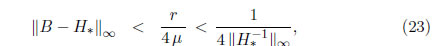
To prove that is well defined, we must show that B−1 exist. For this, we consider the inequality

By the continuity of F, for all > 0 exist  > 0 such that ,
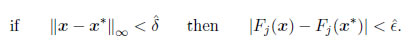
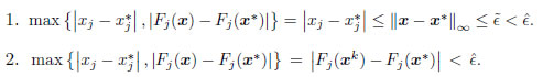
 =min{,}. If x−x*∞ < then | Fj(x)−Fj(x*)| < . On the other hand,
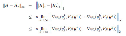
We consider the two possibilities for this maximum:

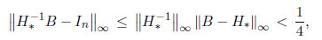
H*−1B−In ∞ < 1. By Banach's Lemma2 there exists B−1 and therefore the function is well defined. Moreover, 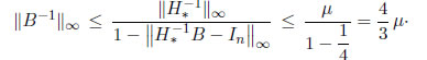
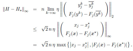
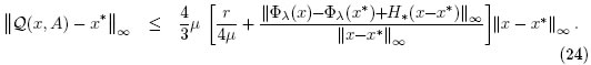
The second part of the proof is to show (19). For this, we subtract x* in (18), we apply ·∞ and perform some algebraic manipulations.
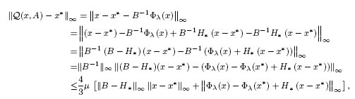
then we obtain,
On the other hand, for H ∂Φλ(x).
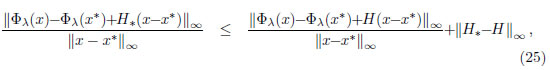
x−x*∞ < ϵ2 then 
 exist ϵr > 0 such that, if x−x*∞ < ϵr then
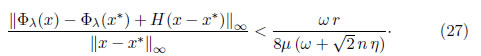
,ϵr}. If x−x*∞ < ϵ0, and A−F′(x*)∞ < δ0 then, from (27), (22), (25) and (24), 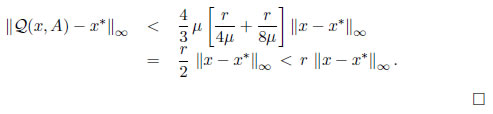
The following theorem is analogous to the theorem of the two neighborhoods of differentiable case [10], which guarantees linear convergence of the proposed algorithm. The name of the two neighborhoods is due to, in its assumptions, it requires two neighborhoods, one for the solution which should be the starting point, and the other for the Jacobian matrix of F at the solution which should be the initial approach.
Theorem 1 Let H1-H3 be verified and let r (0,1), then there exist positive constants ϵ1 and δ1 such that, if x0−x*∞ ≤ ϵ1 and Ak−F′(x*)∞ ≤ δ1, for all k, then the sequence {xk} generated by xk+1=xk−Bk−1Φλ(xk), with Bk the matrix whose rows are defined by (15) is well defined, converges to x* and satisfies

We consider the function (18). Thus,

Given r (0,1), let ϵ1 (0,ϵ0) and δ1 (0, δ0) where ϵ0 and δ0 are the positive constants given by the Lema 3.2. We will use induction on k in the proof of this theorem.
- For k= 0. If x0−x*∞ ≤ ϵ1 ≤ ϵ0 andA0−F′(x*)∞ ≤ δ1 ≤ δ0 then x1 = (x0,A0) is well defined and satisfies

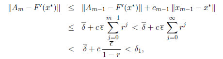
- Induction hypotheses: we assume that for k = m−1,
then xm=xm−1
 Φλ(xm−1), is well define, and
Given that
x0−x*∞ < ϵ1, then 
and from the assumption
Am−F′(x*)∞ ≤ δ1, we have for the Lemma 3.2 that xm+1 is well defined and satisfies 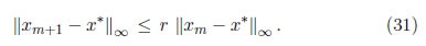
Therefore, we conclude that (28) is true for all k=0,1,…. 
We observe that in the proof of Theorem 3.1 we used the infinity norm. Therefore, if ek = xk−x* is the error related to any other norm, then ek ≤ α rke0, where α is a positive constant that does not depend on k, and r is as in Theorem 3.1.
Among the standard theorems of thequasi Newton theory to systems of nonlinear equations is the theorem known as Dennis-Moré condition [21] which gives a sufficient condition for superlinear convergence. The following theorem is analogous to the theorem just mentioned and it will be useful in the next section to prove superlinear convergence of Algorithm 1. In his proof, we use · = · ∞ but, we recall that superlinear convergence results are norm-independent.
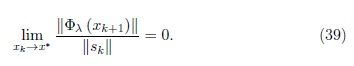
Theorem 2 Let H1-H3 be verified and that, for some x0, the sequence {xk} generated by xk+1=xk− Φλ(xk) converges to x*, with Bk given by (15) and H* = H(x*). If
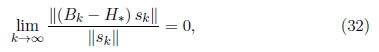
where Sk=xk+1−xk, then the sequence {xk} converges superlinearly to x*.
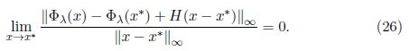
As we mentioned above, Φλ is semismooth in x*, thus
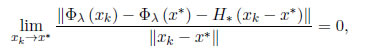
∂Φλ(x*). As Φλ( x*) = 0, then 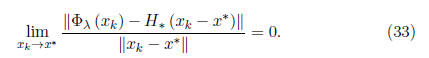

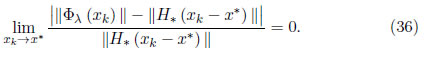
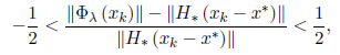
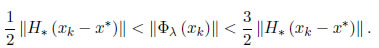
By the limit definition, in particular for  , there exists ϵ > 0, such that if xk−x* < ϵ then,
since


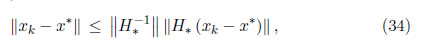
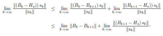
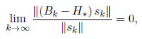
Applying a norm and the triangle inequality, we obtain

thereby

From (3.2), (37) and (16)
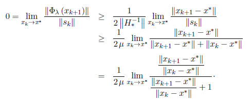
Therefore,
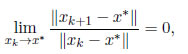
i.e., the sequence {xk} converges superlinearly to x*.
4 Least change secant update family for solving Φλ (x)=0.
The quasi-Newton methods differ in how to update the matrix Ak at each iteration. Among the ''practical'' quasi-Newton algorithm are those that are called least change secant methods, in which the updating of Ak, named Ak+1, must satisfy the secant equation [10] given by Ak+1(xk+1−xk) = F(xk+1)−F(xk) and its change (measured in some norm) relative to Ak must be minimum. Requiring that secant equation and a minimum change are satisfied between two consecutive updates makes the sequence of matrices {Ak } have a property known as bounded deterioration [10] [8], which guarantees that the matrices of the sequence remain in a neighborhood of F′(x*). This is essential to demonstrate local and linear convergence. Thus, at each iteration of the least change secant algorithm, the vectors xk and xk+1 defined the set V by

Given that we need the matrix in V ''nearest'' Ak, it is natural to think of the orthogonal projection of this matrix on V, named PV (Ak) = Pxk,xk+1 (Ak). Given that
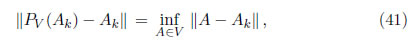
V. This projection is unique because V is a convex set. Therefore, 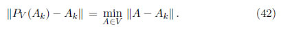
Thus, Ak+1 = PV(Ak).
Different least change secant updates are obtained by varying the matrix norm n×n or the subspace S, producing the family of least change secant update methods. For example, ''Good'' Broyden update,''Bad'' Broyden update [22], Schubert update [23] andSparse Schubert update [23].
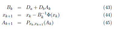
Algorithm 2 Assume that x0 and A0 are arbitrary. xk+1 and Ak+1 for k=0,1,..., are generated as follows:

In order to develop the theory of convergence of the least change secant update methods generated by Algorithm 2we will assume an additional Assumption.
H4. For all x,z in a neighborhood x*, there are A V(x,z) and α1 > 0 such that
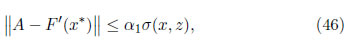
where σ(x,z)=max{x−x*,z−x*}.
5 Additional convergence results
In the next lemma, we show that a matrix generated using the rule (45) to update the matrix Ak may deteriorate, but in a controlled way.
Lemma 5 Let H1-H4 be verified and let A+ be the orthogonal projection of A on the set V(x,z) and  the orthogonal projection of F′(x) on V(x,z) then A+ −F′(x) ≤ A−F′(x)+α2σ(x,z), where α2 > 0 and σ(x,z)=max{x−x*,z−x*}.
Lemma 5. 2 Let assumptions H1-H4 be verified. Then there exists c > 0 such that

whenever the vectors x and y belong to a neighborhood of x*, with y−x* ≤ x−x* and the matrix A in a neighborhood of F′(x*).
The two previous lemmas (see proofs in [16] and [24], respectively) and assumptions H1-H4 are central to ensuring the following result.
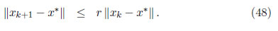
Theorem 5. 1 Let H1 - H4 be verified and that the sequence {Ak} is generated by (45). Given r (0,1), there exist positive constants  and
and  such that if x0−x* ≤ and A0 −F′(x*) ≤ , the sequence {xk} generated by xk+1 = xk−
 Φ(xk) is well defined, converges to x* and, for all k=1,2,…,
Let (0,δ1). We can choose (0,ϵ1) with
, are the following. 1. IfThus, in either case, it is possible to choose< ϵ1, the constant
·
2. If
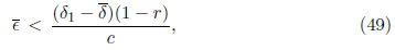
in (0,ϵ1) ∩  . Then, from (49)
1. For k=0, if2. We assume that for k=m−1, if
3. From (51) and (47)
4. From (47),
where
and ci is the constant of Lemma 5.2. Thus, from Lemma 3.2, xm+1 is well defined and satisfies

Lemma 5. 3 We assume the Assumptions H1 - H4 are verified and let the sequence { Ak} be generated by (45). There are positive constants y such that, if x0−x* ≤ and A0−F′(x*) ≤ , and the sequence {xk} is generated by xk+1xk−Bk−1Φ( xk), with Bk defined by (15), then
With this result (See proof in [16]), we can derive sufficient condition to have super linear convergence as shown by the next Theorem.
Theorem 5.2. Let the Assumptions H1-H4 and let the sequences {xk} and { Ak} be generated by the Algorithm 2 and xk=x*. If
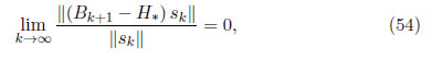
The proof follows in a straightforward way from Theorems 4.2 and 4.3.
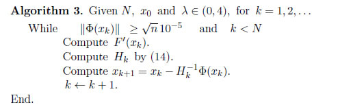
6 Some numerical experiments
In this section, we analyze numerically the local behavior of the family of least change secant update methods introduced in Section 2. For this, we compare our algorithms with the Generalized Newton method proposed in [6]. The Algorithm 3 is a Generalized Newton type method. It uses at each iteration, the matrix Hk (defined in the previous section) which uses the Jacobian Matrix of F.
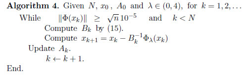
The Algorithm 4, which is a least secant change type method is based on the Algorithm 2 that we proposed at Section 3. For updating the matrix Ak, in each iteration, we use the four formulas: ''Good'' and ''bad'' Broyden, Schubert and Sparse Schubert, whereby we have four versions of Algorithm 4.
For all the tests, we use the software MATLAB®. We use 8 test problems for nonlinear complementarity, four of which we chose from a list proposed, [14] and which are considered ''hard problem''. These are Kojima-Shindo (application to Economic Equilibrium [25]), Kojima-Josephy, Nash-Cornout (application to the Game Theory harker) and Modified Mathiesen (application to Walrasian Economic Equilibrium [26]) problems. We generate the four remaining problems like in [27]; for this, we define F : n→n by,
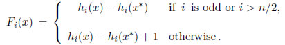
n is a degenerate solution and the functions hi are given by Luksan [18], namely,Trigonometric system, Exponential trigonometric, tridiagonal and Rosenbrock. We use the same stopping criteria proposed in [28]. We choose the parameter λ:=λmin for using in the Algorithms 3 and 4 as follows
For the numerical test, we vary λ in the interval (0,4) from λ = 10−3 to λ = 3.999 with increments of 10−3. Of all these values of λ, that for which the generalized Newton method converges in less iterations, we call it λmin , and we use it as the parameter λ in Algorithms 3 and 4. The initial approximations are the same as in [14] and [18].We vary λ in the interval (0,4) from λ = 10−3 to λ = 3.999 with increments of 10−3.
We use the generalized Newton method (Algorithm 3) with each of these values of λ.
We called λmin to the value of λ for which the generalized Newton converges in fewer iterations.
Table 1 presents the results of our numerical tests. Its columns contains the following information: Problem means the problem name, n is the dimension problem, λmin is the value of λ for which the Algorithm 3 converges in fewer iterations. We also include a column with the algorithm and the secant update used. Thus, GN means Generalized Newton; SSU, BBU, SU and GBU means Algorithm 4 with the Sparse Schubert Update, ''Bad'' Broyden Update, Schubert Update and the ''Good'' Broyden Update, respectively. A − sign means divergence.
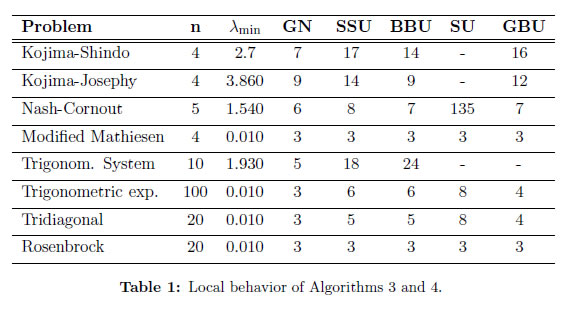
From Table 1, we observe that, for these preliminary numerical tests, the Algorithm 4 that we proposed for solving the NCP has good local behavior. In particular, we highlight the Modified Mathiesen problem, in which each method converges with the same number of iterations but to different solutions to the problem.
7 Conclusions
In this paper, we propose a quasi-Newton method for solving the nonlinear complementarity problem when this is reformulated as a nonlinear system of equations. This method can be useful when the derivatives of the system are very expensive or difficult to obtain. Moreover, we generated a family of least change secant update methods that, under certain hypotheses, converge local and superlinearly to the solution of the problem.
Some numerical experiments shows a good local performance of this algorithm, but it is necessary more numerical tests using others well-known LCSU methods such as Column Updating method [29] Inverse Column Updating method [30]. It is necessary to incorporate a globalization strategy to the algorithm proposed and to develop theoretical and numerical analysis of the global algorithm.
Acknowledgements
The authors would like to thank the Universidad del Cauca for providing time for this work through research project VRI ID 3908 and anonymous referees for constructive suggestions to the first version of this paper, which allowed us to improve the presentation of this article.
Footnotes:
1 We consider the same sequence of [20] which is used for the theoretical developments with the Fischer function.
2 Let · a matrix norm induced in n ×n, A and C n×n. If C is non singular and In−C−1A < 1 then A is non singular and A−1 ≤  ·
·
References [ Links ]
[2] M. Kostreva, ''Elasto-hydrodynamic lubrication: A non-linear complementarity problem,'' International Journal for Numerical Methods in Fluids, vol. 4, no. 4, pp. 377-397, 1984. [ Links ]
[3] A. Chen, J.-S. Oh, D. Park, and W. Recker, ''Solving the bicriteria traffic equilibrium problem with variable demand and nonlinear path costs,'' Applied Mathematics and Computation, vol. 217, no. 7, pp. 3020-3031, 2010. [ Links ]
[4] M. C. Ferris and J.-S. Pang, ''Engineering and economic applications of complementarity problems,'' SIAM Review, vol. 39, pp. 669-713, 1997. [ Links ]
[5] L. Yong, ''Nonlinear complementarity problem and solution methods,'' in Proceedings of the 2010 international conference on Artificial intelligence and computational intelligence: Part I. Springer-Verlag, 2010, pp. 461-469. [ Links ]
[6] L. Qi, ''Convergence analysis of some algorithms for solving nonsmooth equations,'' Math. Oper. Res., vol. 18, no. 1, pp. 227-244, 1993. [ Links ]
[7] V. L. R. Lopes, J. M. Martínez, and R. Pérez, ''On the local convergence of quasi-newton methods for nonlinear complementary problems,'' Applied Numerical Mathematics, vol. 30, pp. 3-22, 1999. [ Links ]
[8] C. G. Broyden, J. E. Dennis, and J. J. Moré, On the Local and Superlinear Convergence of Quasi-Newton Methods, ser. PB 211 923. Department of Computer Science, Cornell University, 1972. [ Links ]
[9] D.-H. Li and M. Fukushima, ''Globally convergent broyden-like methods for semismooth equations and applications to vip, ncp and mcp,'' Annals of Operations Research, vol. 103, no. 1-4, pp. 71-97, 2001. [ Links ]
[10] J. E. Dennis and R. B. Schnabel, Numerical Methods for Unconstrained Optimization and Nonlinear Equations. Society for Industrial and Applied Mathematics, 1996. [ Links ]
[11] R. Pérez and V. L. R. Lopes, ''Recent applications and numerical implementation of quasi-newton methods for solving nonlinear systems of equations,'' Numerical Algorithms, vol. 35, pp. 261-285, 2004. [ Links ]
[12] C. Ma, ''A new smoothing quasi-newton method for nonlinear complementarity problems,'' Applied Mathematics and Computation, vol. 171, no. 2, pp. 807-823, 2005. [ Links ]
[13] S. Buhmiler and N. Kreji\'c, ''A new smoothing quasi-newton method for nonlinear complementarity problems,'' Journal of Computational and Applied Mathematics, vol. 211, no. 2, pp. 141 - 155, 2008. [ Links ]
[14] J.-S. Pang and L. Qi, ''Nonsmooth equations: Motivation and algorithms,'' SIAM Journal on Optimization, vol. 3, no. 3, pp. 443-465, 1993. [ Links ]
[15] C. Kanzow and H. Kleinmichel, ''A new class of semismooth newton-type methods for nonlinear complementarity problems,''Comput. Optim. Appl., vol. 11, no. 3, pp. 227-251, 1998. [ Links ]
[16] F. E. Arenas A., ''Métodos secantes de cambio mínimo,'' Master's thesis, Universidad del Cauca, 2013. [ Links ]
[17] J. M. Martínez, ''Practical quasi-newton methods for solving nonlinear systems,'' Journal of Computational and Applied Mathematics, vol. 124, no. 1, pp. 97 - 121, 2000. [ Links ]
[18] L. Luksan, ''Inexact trust region method for large sparse systems of nonlinear equations,'' Journal of Optimization Theory and Applications, vol. 81, pp. 569-590, 1994. [ Links ]
[19] F. H. Clarke, Optimization and Nonsmooth Analysis. Society for Industrial and Applied Mathematics, 1990. [ Links ]
[20] T. De Luca, F. Facchinei, and C. Kanzow, ''A semismooth equation approach to the solution of nonlinear complementarity problems,'' Mathematical Programming, vol. 75, pp. 407-439, 1996. [ Links ]
[21] J. E. Dennis, Jr. and J. J. More, ''A characterization of superlinear convergence and its application to quasi-newton methods,''Mathematics of Computation, vol. 28, no. 126, pp. 549-560, 1974. [ Links ]
[22] C. G. Broyden, ''A Class of Methods for Solving Nonlinear Simultaneous Equations,'' Mathematics of Computation, vol. 19, no. 92, pp. 577-593, 1965. [ Links ]
[23] T. F. Coleman, B. S. Garbow, and J. J. More, ''Software for estimating sparse jacobian matrices,'' ACM Trans. Math. Softw., vol. 10, no. 3, pp. 329-345, Aug. 1984. [ Links ]
[24] J. M. Martínez, ''On the relation between two local convergence theories of least change secant update methods,'' Mathematics of Computation, vol. 59, no. 200, pp. pp. 457-481, 1992. [ Links ]
[25] M. Kojima and S. Shindoh, Extensions of Newton and Quasi-Newton Methods to Systems of PC 1 Equations, ser. Research reports on information sciences. Inst. of Technology, Department of Information Sciences, 1986. [ Links ]
[26] L. Mathiesen, ''An algorithm based on a sequence of linear complementarity problems applied to a walrasian equilibrium model: An example,'' Mathematical Programming, vol. 37, pp. 1-18, 1987. [ Links ]
[27] M. A. Gomes-Ruggiero, J. Martnez, and S. A. Santos, ''Solving nonsmooth equations by means of quasi-newton methods with globalization,'' Recent Advances in Noonsmooth Optimization, World Scientific Publisher, Singapore, pp. 121-140, 1995. [ Links ]
[28] R. Pérez M., ''Algoritmos para complementariedade não lineal e problemas relacionados,'' Ph.D. dissertation, IMECC, UNICAM, Campinas, Brazil, Dezembro 1997. [ Links ]
[29] J. M. Martínez, ''A quasi-newton method with modification of one column per iteration,'' Computing, vol. 33, no. 3-4, pp. 353-362, 1984. [ Links ]
[30] J. M. Martínez and M. C. Zambaldi, ''An inverse column-updating method for solving large scale nonlinear systems of equations,''Optimization Methods and Software, vol. 1, no. 2, pp. 129-140, 1992. [ Links ]
