


Servicios Personalizados
Revista
Articulo
 Inglés (pdf)
 Articulo en XML
 Referencias del artículo
 Enviar articulo por email
Indicadores
-
 Citado por SciELO
 -
 Accesos
Links relacionados
-
 Citado por Google
 -
 Similares en
SciELO
Similares en
SciELO -
 Similares en Google
Compartir

 Permalink
Ingeniería y Ciencia
versión impresa ISSN 1794-9165
ing.cienc. vol.11 no.21 Medellín ene./jun. 2015
https://doi.org/10.17230/ingciencia.11.21.2
ARTÍCULO DE REVISIÓN
doi: 10.17230/ingciencia.11.21.12
Methods Employed in Optical Emission Spectroscopy Analysis: a Review
Métodos empleados en el análisis de espectroscopía óptica de emisión: una revisión
D. M. Devia 1, L. V. Rodriguez-Restrepo 2 and E. Restrepo-Parra 3
1 Universidad Tecnológica de Pereira, Pereira, Colombia, dmdevian@utp.edu.co.
2 Universidad Nacional de Colombia, Sede Manizales, Colombia, lvrodriguezr@unal.edu.co .
3 Universidad Nacional de Colombia, Sede Manizales, Colombia ereatrepopa@unal.edu.co.
Received: 15-06-2014 | Acepted: 25-09-2014 | Online: 01-30-2015
PACS: 52.25.Dg, 31.15.V
Abstract
In this work, different methods employed for the analysis of emission spectra are presented. The proposal is to calculate the excitation temperature (Texc), electronic temperature (Te) and electron density (ne) for several plasma techniques used in the growth of thin films. Some of these techniques include magnetron sputtering and arc discharges. Initially, some fundamental physical principles that support the Optical Emission Spectroscopy (OES) technique are described; then, some rules to consider during the spectral analysis to avoid ambiguities are listed. Finally, some of the more frequently used spectroscopic methods for determining the physical properties of plasma are described. OES; plasma parameters; Key words: elemental determination; line intensity; broadening; shifting
Resumen
En este trabajo se presentan diferentes métodos empleados para el análisis de espectros ópticos de emisión. El propósito es calcular la temperatura de excitación (Texc), temperatura electrónica (Te) y densidad electrónica (ne) empleando diversas técnicas usadas en el crecimiento de películas delgadas. Algunas de estas técnicas incluyen magnetron sputtering y descargas n arco. Inicialmente, se describirán algunos principios fundamentales que soportan la técnica de Espectroscopía Óptica de Emisión (EOE); posteriormente, se considerarán algunas reglas que deben considerarse para el análisis de espectros con el fin de evitar ambigüedades. Finalmente, se presentarán algunos d los métodos espectroscópicos más determinar las propiedades físicas de plasmas.
Palabras clave: OES; parámetros de plasma; determinación elemental; intensidad de lineas; ensanchamiento; corrimiento
1 Introduction
Plasma diagnostics are the techniques used to obtain information about the nature (properties) of plasma, such as the chemical compositions and species of the plasma, density of the plasma, plasma potential, electron temperature, ion/electron energy distributions, ion mass distributions and neutral species [1],[2]. Some of the techniques employed for the characterization of plasma include the Langmuir probe [3],[4], interferometry [5], mass spectroscopy [6], the Thompson dispersion method [7] and optical emission spectroscopy (OES) [8]. The most direct plasma characterization technique that requires low theoretical analysis is likely the Thompson dispersion method; however, the spectroscopy technique is the simplest if the instrumentation permits the use of it. Spectroscopic methods for plasma diagnostics are the least perturbative, and for the evolution of the plasma parameters, they study the emitted, absorbed or dispersed radiation [9]. Generally, spectral diagnostic methods attempt to establish relationships between the plasma parameters and the radiation features, such as the emission or absorption intensity and the broadening or shifting of the spectral lines. The applicability of these methods depends on the system that is being studied because some of the techniques are general and others are not easily applied in total and local thermodynamic equilibrium. Many studies in the literature on plasma parameters use the OES technique, which can be applied in many fields, from spatial plasmas [10] to laboratory experiments such as nuclear fusion [8] and plasma-assisted material production [11]. OES is a very useful technique in materials processing because the plasma features can be correlated with the characteristics of the material. Furthermore, OES is employed as a control tool during the process to control contamination and to enable time and spatial monitoring of the plasma. G. Zambrano and E. Restrepo et al [12] performed plasma studies on a magnetron sputtering discharge implemented for the production of WC/DLC multilayers with a mixture of Ar/CH4. The information gained from the plasma spectrum obtained during the production process allowed the species contained in the plasma and their densities to be determined. These parameters were subsequently correlated with the structure and composition of the films. E. Restrepo and A. Devia analyzed the properties of plasma that was produced in a pulsed vacuum arc system. The system was used to grow TiN coatings. In this work, the electron temperature and density were determined using spectroscopic techniques, including the lines-continuum ratio, line-line ratio and Stark broadening techniques. L.A García et al [13] studied the parameters of a pulsed arc plasma using the electrostatic probe and OES techniques. This plasma was used for growing DLC coatings. Values of Te and ne were obtained by both techniques. H. Jiménez et al [14] characterized the plasma used in the production of TiO2 thin films by the pulsed arc technique. Again, different spectroscopic methods were used to determine the parameters of the plasma. Many studies performed by other authors can be found in the literature. For example, Yong M. Kim et al [15] studied the nitrogen behavior in a DC plasma nitriding process. To establish a suitable process control, the densities of the active nitrogen species must be monitored because they are responsible for the ferro/metal reactions. Using OES, the authors observed the nitrogen concentration with respect to hydrogen. Hassan Chatei et al [16] studied a microwave H2 − CH4 −N2 plasma used for the deposition of diamond films in continuous and pulsed mode using the OES technique. In the continuous mode, an actinometrical OES technique was used for determining the tendency of H, CH and CN species concentration. The authors concluded that important information about the transition phases and the different excitation processes can obtained using the optical measurements, and the results indicated that the electronic excitation process was predominant. Because of the great utility of spectroscopic techniques in the study of plasma and its applications, some important basic concepts are addressed in this document, which provides insight on some of the most widely used spectroscopic methodologies for the characterization of plasma. These methodologies include line-to-line relationships and line broadening. To use spectroscopic techniques in an appropriate manner, it is necessary to have certain expertise and knowing some useful tips for identifying the species, choosing the lines for the calculations and selecting the most suitable method. By using these methods, the substances present in the plasma can be identified, and parameters such as the excitation temperature (Texc), electron temperature (Te) and electron density (ne) can be determined. In addition to the description of the methods, examples of the application of the methods are presented in this work.
2 Fundamental concepts
2.1 Total thermodynamic equilibrium
The physical state of homogeneous plasma contained in a vessel with isothermal walls at a temperature T can be described with the help of certain macroscopic variables (temperature, pressure and the concentration of various components) without knowing all of the microscopic processes that are occurring in detail. In this state, the plasma is in thermodynamic equilibrium. When the equilibrium state is reached, a certain number of laws that enable the determination of the state of matter and the radiation inside the vessel can be obtained using statistical mechanics [17]. For different plasma species, the Maxwell, Boltzmann and Saha laws govern the velocity distribution function of the particles, the excited state and the ionization degree, respectively. Planck's law governs the spectral distribution of the radiation.2.2 Maxwell's law
This law describes the distribution of the particles that compose the plasma with respect to their velocities. The density, dN, of any type of particles that have velocities in the v+dv range can be described as dN=Nf(v)dv, where Nis the density of the species of particles considered and f(v) is the Maxwell velocities distribution function:
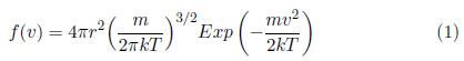
where k is Boltzmann's constant, which has a value of 1.38 10 − 23J/K m is the mass of the particle and T is the temperature [18].
2.3 Boltzmann's law
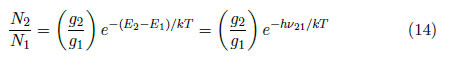
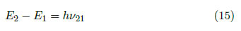
Boltzmann's law enables the determination of the excited state population of an atom or a molecule. Let N1 and N2 be the densities of particles of a given species, which are distributed into 1 and 2 levels, respectively. In agreement with Boltzmann's law,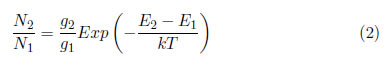
where E1 and E2 are the energies of levels 1 and 2, g1 and g2 are the statistical weights of the energies of levels 1 and 2 and T is the temperature.
The statistical weight or state density (g1) of a state of energy E1 is related to the quantum number J1, which corresponds to the total kinetic moment of the i-th level through the relationship gi = 2Ji + 1 [19].
It is interesting to express the density of particles, Ni, of the i-th level as a function of the total relative density of all levels sum Ni = N. Using , the following equation was obtained
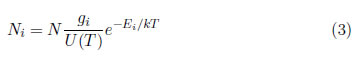
where T is the average temperature of the electrons in the i-th energy state and the partition function [17], which is written as:
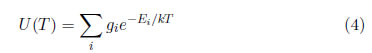
This function acts like a normalization factor that ensures the fulfillment of equation (2).
2.4 Saha equation
When Boltzmann's law is generalized for continuous states (2) that are located far from the ionization state, the Saha equation can be obtained. This equation is related to the electronic density (Ne), the density (Nz) of the ions with charge Ze and the density (Nz+1) of the ions with charge (Z+1)e, as follows: [20]: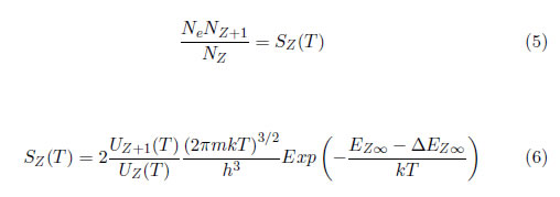
Uz+1T and UzT are the partition functions of the ions with charge (Z+1)e and Ze, respectively, h is Planck's constant (6.626 ×10⁻³⁴ J.s), is the mass of the electron (9.109×10⁻³¹ Kg), Ez∞ is the ionization energy and is the minimum ionization energy.
2.5 Local thermodynamic equilibrium
The total thermodynamic equilibrium conditions are primarily only presented in stellar bodies where large volumes at high temperatures can be observed. Therefore, in laboratory plasmas, ''local thermodynamic equilibrium-LTE'' can be considered. In laboratory plasmas with small dimensions, a significant portion of the emitted radiation escapes without being reabsorbed (optically thin plasmas), the spectral intensity does not follow Plank's law [21], and the excited state population is no longer governed by Boltzmann's distribution. The fundamental level is overcrowded, whereas the higher levels are weakly populated due to the absence of radiation. However, the problem is significantly simplified when the electron density is high such that the electron collisions are completely responsible for all of the excitation process, de-excitation, ionization and recombination.Under these conditions, it is possible to use the LTE concept. In this concept, the electron distribution function is assumed to be Maxwellian at each point in the plasma with respect to the electronic temperature (Te) [22]. Ocassionally, considering partial local thermodynamic equilibrium (PLTE) is better. For a large number of elements and for hydrogen, the transversal collision sections decrease and transition probabilities increase as the fundamental level is reached [23]. For the LTE concept to hold in a plasma, the collisions with electrons must dominate over the radiative processes, which requires a sufficiently large electron density. A criterion proposed by McWhirter [24] was based on the existence of a critical electron density where the collisional rates are at least ten times the radiative rates. For an energy gap difference (∆E) between the transition levels, the criterion for LTE is [25]: Ne ≥ 1.6x10¹²T1/2(∆E)3 cm− 3.
2.6 Partial local thermodynamic equilibrium
For a fixed ne, the LTE condition expressed in eq. (5) can be fulfilled by high-energy excited levels and not by low-energy levels. If a level n' exists where the two rates are the same, then the plasma is in partial LTE (pLTE), where the levels n>n' and the free electrons are in equilibrium with each other while the levels n<n' are not. In this case, the atomic state distribution function is divided in two parts, as follows: the upper side that contains the high-energy levels n>n', which are easily thermalized, follow a Boltzmann distribution at the temperature Texc=Te and are related to the ion population by the Saha relation, and the bottom side, where the energy gap with the continuum is too large and the associated levels do not follow the Saha–Boltzmann distributions. It is obvious that for plasmas in pLTE, the experimental determination of Texc using a Boltzmann plot obtained by considering all of the spectral lines will result in Texc values being different from Te [26].
3 Spectral line characteristics
3.1 Spectral line intensity
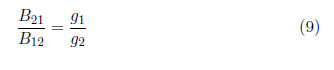
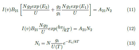
An emission line is defined as the energy emitted per second and it depends on the probability of transitioning between the two involved energy levels and their electron population. In thermodynamic equilibrium, the population distribution of the i−th level, Ni(Ei), is given by the Boltzmann distribution, which is presented in eq. (2). In a stationary field, the total absorption rate, N1B12I(v), that represents the number of absorbed photons per volume per second must be equal to total emission rate N2B21I(v) + N2A21 because of the energy conservation law. N1 and N2 represent the population of levels 1 and 2, I( ν) is the spectral intensity, and A21, B21 and B12 are the Einstein coefficients of spontaneous emission, induced emission and absorption, respectively [27].

The Einstein coefficients can be written as , y
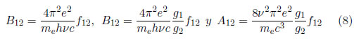
where c is the speed of light and f12 is the strength of the oscillator; therefore,
then,
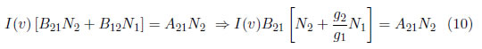
By replacing eq. (3)
By using eq. (2) for two different transitions and establishing a relationship between the transitions, the following is obtained:
where
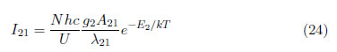
where I21 is the line intensity and v21 is the transition frequency. By replacing (2) and evaluating eq. (15) with i = 2, the spectral line intensity can also be described as:
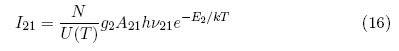
where g2 is the density of states, E2 is the upper level energy and T is the excitation temperature.
3.2 Spectral line broadening
Several factors result in the broadening of the spectral lines. This broadening can be Lorentzian, Gaussian or Voigt (a mixture of Lorentzian and Gaussian), as shown in Figure 1(a). The broadening depends on the phenomena responsible for the broadening. In the following, the most important factors for broadening are explained [28].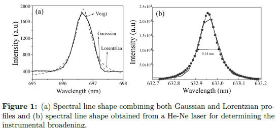
3.3 Natural broadening
During a transition, the electron provides the energy that corresponds to the difference between two atomic levels. According to the Heisenberg uncertainty principle and the small lifetime of the excited states, the energy levels are not exactly defined, which results in the energy of the emitted photon presenting an error [29]. As is well known, the transition energy and frequency are directly related, which produces an uncertainty in the frequency that is reflected in the line broadening. The profile generated as a consequence of natural broadening is given by:
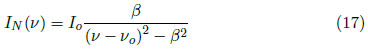
where IN(ν) is the spectral line intensity due to the natural transition energy, Io is the maximum intensity, νo is the central frequency and β is a constant. The natural broadening is Lorentzian type, which is characterized by greater tails. This broadening has typical values on the order of 0.01 pm in units of wavelength.
3.4 Doppler broadening
The random movement of emitted atoms relative to the spectrometer causes a broadening known as Doppler or sometimes called temperature broadening, which introduces a Gaussian profile [30].
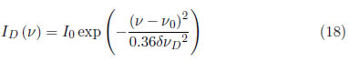
where δνD is the broadening of the spectral line due to the Doppler effect given by:

where ID(ν) is the line intensity, R is the ideal gas constant (8.31451[J/K.mol]) and M is the mass of the atom or ion.
3.5 Pressure broadening, coalitional or stark broadening
Atomic collisions can produce a Lorentzian profile in the lines. The Stark effect results in a shift or division of the spectral lines into several components due to the presence of an electrical field. This effect is analogous to the Zeeman effect, which also produces broadening but is caused by a magnetic field. The Stark effect is produced by collisions of charged particles that have a permanent, strong dipole moment. A strong and chaotic electric field produces Stark broadening, and a static electric field induces shifting. The pressure dependence can be described from the damping due to collisions [31].
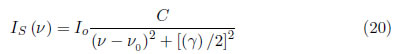
where Is(v) is the line intensity and C is a constant
3.6 Instrumental broadening
Because any measured light may pass through the slit of the spectrometer, a diffraction effect that broadens the lines is produced. As the slit width increases, the resolution decreases. In addition, the lenses used in the instrumentation also introduce a measurement error, which results because these lenses normally have certain aberration. The instrumental line profile has a Lorentzian shape, and it can be measured by replacing the plasma with a Geissler tube at low pressure, which is commercially available, or by simply using a monochromatic light (laser). Figure 1(b) presents an example of a profile measured using a He-Ne laser [32].3.7 Real broadening
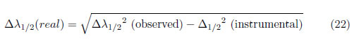
The real broadening of a spectral line is simply the convolution or sum of all of the broadenings produced by the different phenomena. In other words, the real line shape is a convolution of the Lorentzian and Gaussian profiles, which is called a Voigt profile. The natural broadening is generally neglected because it is normally several orders of magnitude less than the others. Because some import plasma properties can be determined from the line broadening, examples for calculating the line broadening based on the phenomenon are presented.(i) If a line is primarily broadened by the Stark effect and instrumental broadening, which generates a Lorentzian profile, the real broadening can be approximately obtained from [33]:

where is the Full Width at Half Maximum (FWHM)
(ii) If the line has a predominant Doppler broadening, which has a Gaussian profile, the real width is given by:
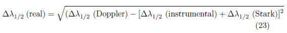
(iii) If the line has contributions from not only the Stark effect but also Doppler broadening, the FWHM can be calculated as
4 Some spectroscopic techniques
4.1 Spectral lines identification
The identification of the spectral lines is very important when studying any substance using optical emission spectroscopic techniques. Not performing a suitable identification produces erroneous results. In some cases, the identification of spectral lines is complicated because of the following reasons:(i) There are some errors introduced by instrumentation that has a certain resolution. For example, if a device has a resolution of 0.2 nm, and the spectral line is theoretically placed at 538.0337 nm (C I – neutral carbon) [33], the spectrometer can present the line between 538.2337 nm and 537.8337 nm.
(ii) Another difficulty caused by the instrumental resolution is the impossibility of separating two lines that have differences that are less than the resolution (instrumental broadening). In this case, the lines overlap and they appear as one line, which makes using signal deconvolution techniques necessary.
(iii) Although the emission wavelength (frequency) values of a substance are like a fingerprint, it does not avoid the presence of radiation emission of several substances at closer wavelengths with differences (∆λ) less than the instrument resolution. For instance, NI (neutral nitrogen) emits radiation at 600.8473 nm, and CI (neutral carbon) emits at 600.718 nm. In this case, ∆λ=0.1293 nm; if the instrument resolution is 0.2 nm, is less than the resolution, which makes determining if the line belongs to carbon or nitrogen impossible. (iv) There are physical reasons that produce a shift in the spectral lines. An example is the shift caused by the Stark effect or by pressure, as was stated previously. To avoid these problems, the spectroscopists may look for solutions that allow these problems to be solved at the moment the spectral lines are identified. Some tips are presented in the following:
Before performing the experiment, collect a spectrum of a light source of a monoatomic substance that belongs to a known element. Use the database and observe the reported lines present in the spectrum. If there is a shift, try to calibrate the equipment until the shift becomes the lowest. Repeat this procedure at the beginning of each experiment. In addition to calibrating the equipment, this procedure will enable you to identify the shift produced by the instrument.
Some transitions between energy levels occur with higher probabilities than others. Therefore, the spectral lines at these wavelengths are intense. If you have doubts identifying one spectral line, especially if it belongs to a certain substance, it could be expected that the other lines of this substance with high intensity appear in the spectrum.
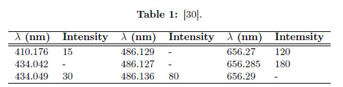
An example is presented in the following. Hydrogen emits several lines at the wavelength shown in Table 1. In this table, the relative intensities of these lines are also included. The lines at 434.042, 486.129, 486.127 and 656.29 nm [33], [34] can likely be hidden because of noise or by other lines. Nevertheless, the lines at 410.176, 434.049, 486.136, 656.27 and 656.285 nm [33], [34] appeared with significant intensities and could be identified in the emission spectrum when hydrogen was present in the analyzed substance.
To ensure that the line set belongs to certain material, the distances between the lines may be measured; they have to be compared with the distances of the lines in the database and they may be similar. Despite the lines shifting and broadening caused by different factors, the distances between the lines must be similar to those reported in the database.
When lines that do not belong to any of the expected substances appear in the spectrum. For example, in a reactor, some hydrocarbides, such as methane and acetylene, are introduced, and the spectrum is expected to contain C, H, CH, and so on. If there are other elements or substances, they are likely contaminants such as oxygen nitrogen steel or cobalt, some of which belong to the material employed in the reactor construction and others, such as those in the air that cannot be totally evacuated during the vacuum process.
For measuring the line broadenings that are different from the instrumental broadening and thus determining several physical characteristics of plasma from these broadenings, a high-resolution instrument is required, if possible, at scales beyond nanometers.
5 Experimental setup
In this work, results from two different experiments are presented. The first one consists of the production of YBaCuO coatings using the magnetron sputtering rf technique. The sample holder enables the substrate temperature to be varied by changing the resistance. In this case, the temperature was maintained at 550 ºC. The chamber was connected to an rf power supply. The target was YbaCuO, and the working pressure was 0.006 mbar with different concentrations of Ar/O2. The rf power supply was varied between 50 and 150 W. The second experiment consists of a pulsed vacuum arc system with a RLC circuit, O2 working gas at a pressure of 2.4 mbar and a discharge voltage of 200 V. In the first case, an ORIEL model 77480 spectrometer of 1/4 m was employed. A diffraction grating of 2400 lines/mm and a 25 micron slit were used. For obtaining the data, a CCD camera composed of 1024 ×256 photodiodes, which allows recording average wavelength ranges of 50 nm with a resolution of 0.1 nm, was used. With this array, spectra from 200 nm to 1000 nm can be obtained. In the second case, a high-resolution HR spectrometer with a HC1 diffraction grating of 1200 line/mm with an entrance slit of 20μm. This instrument records spectra at wavelengths between 100 nm and 1100 nm and has a resolution of approximately 1.5 nm. The plasma is produced by a discharge with a mixture of argon and nitrogen as a working gas, which is similar to a conventional magnetron sputtering system. The working power was 200 W, the pressure was 5x10 − 3 mbar, and the argon flow was 2.8xcm3/min.
6 Results and discussion
6.1 Atomic and molecular spectral lines
In many spectra, lines from neutral atoms, atomic ions, molecules and molecular ions can appear. With the naked eye, lines that belong to atoms or molecules (normally called molecular bands) can be differentiated. In Figure 2(a) and Figure 2(b), two spectra from a discharge generated for producing YBaCuO coatings by the magnetron sputtering technique are presented. Figure 2(a) shows a spectrum with narrow and symmetric lines that corresponds to neutral argon. The symmetry of these lines is caused by transitions between two atomic levels, and despite the fact that they have a finite broadening because of the uncertainty principle, this contribution can be neglected. In contrast, Figure 2(b) presents a spectrum generated during the same process. The asymmetry and the high broadening of the lines indicate that they were produced by molecular transitions of nitrogen (N2) [35], which has strong emission at wavelengths in the ultraviolet range. In this spectrum, the observed lines are wide and asymmetric due to molecules emitted because of not only electron transitions but also rotational and vibrational energy levels at closer frequencies [36], [37]. With a high-resolution spectrometer, each of these bands represented by narrower lines could be identified, and subsequently, the vibrational and rotational energy levels of the molecules could be determined.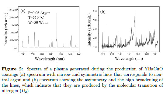
Spectra of a plasma generated during the production of YBaCuO coatings (a) spectrum with narrow and symmetric lines that corresponds to neutral argon and (b) spectrum showing the asymmetry and the high broadening of the lines, which indicate that they are produced by the molecular transition of nitrogen (N2)
6.2 Excitation temperature
To calculate the excitation temperature, the line-to-line ratio method was used [38]. The Boltzmann plot can be used, according to eq. (15). By rewriting eq. (16), the spectral line intensity can be written as:
N, h, c and U are the same for all of the atomic lines; therefore: , and
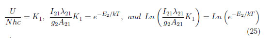
where
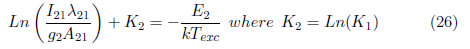
Plotting
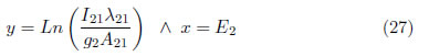
A curve is obtained with a slope of m = − 1 /kTexc This method is widely used in the literature [39]. For obtaining a better understanding, two different transitions between energy states, m-n and p-n, were considered; the first transition occurs between levels m and n, where m is the upper level and n is the level with lower energy. The spectral line intensity is:
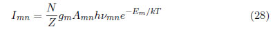
The second transition is between energy levels p and n, where p is the level with upper energy and n is the level with lower energy; the line intensity is given by:
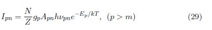
Correlating these spectral lines, the next equation is obtained:
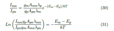
By performing a variable substitution, we obtain: , where
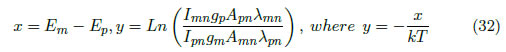
A line with slope -1/kTexc was obtained, and Texc can be subsequently calculated. The excitation temperature, Texc, is defined for a population of particles via the Boltzmann factor. Therefore, the excitation temperature is the temperature where a system with this Boltzmann distribution is expected. However, this parameter only has physical meaning when the system is in local thermodynamic equilibrium [40]. Figure 3(a) presents the plot used for determining the excitation temperature for the experiment conducted at a pressure of 0.04 Ar/0.02 O2 with a substrate temperature of 550 ºC and a power of 80 watts. The excitation temperature, Texc, was 3921.29 K.
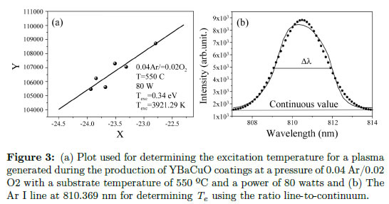
Figure 3(a) Plot used for determining the excitation temperature for a plasma generated during the production of YBaCuO coatings at a pressure of 0.04 Ar/0.02 O2 with a substrate temperature of 550 ºC and a power of 80 watts and (b) The Ar I line at 810.369 nm for determining Te using the ratio line-to-continuum.
6.3 Electron temperature using the line-to-continuum ratio.
The spectral line intensity is given by Eq. (16). The Saha equation can be written as:
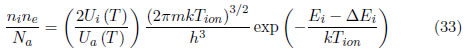
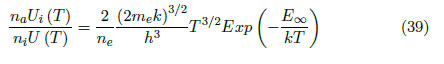
where ni and ne are the ion and electron densities, respectively, Zi, is the ionic partition function, m is the electron mass, Tion is the ion temperature, Ei is the ionization energy and ∆Ei is the lower ionization potential. If the factor N/U(T) is replaced from Eq. (16) to Eq. (34), the following relation is obtained:
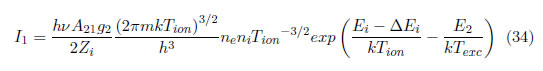
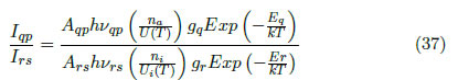
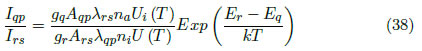
As observed, there are two temperatures. For a system close to local thermodynamic equilibrium (LTE), Tion=Te, can be assumed; nevertheless, Texc can continue being an independent variable that is obtained separately, which allows the other parameters to be calculated. The emission coefficient of the continuum radiation is given by [41], [42]:
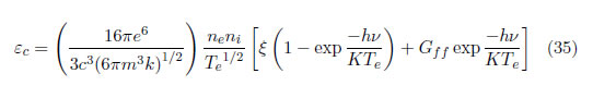
If a relation between (35) and (36) is performed and is expressed as a function of wavelength, then:
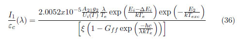
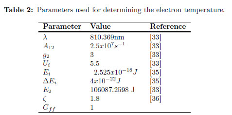
Experimentally, εc is measured closet to the line chosen, and both are presented in arbitrary units. From Eq. (37), Te is calculated. In this case, the experiment implemented for the production of YBaCuO coatings using the magnetron sputtering technique is again employed. For this purpose, choosing a line and finding the corresponding parameter for that line is necessary. Therefore, the Ar I line at 810.369 nm was chosen to obtain the intensity, and the area under the curve could be calculated. In contrast, integrating the continuous intensity is not necessary because it is automatically integrated by the apparatus. In Figure 3(b), the line chosen for determining Te using the ratio line-to-continuum is presented. For calculating the electron temperature, the values listed in Table 2 must be replaced, and the electron temperature obtained previously is also used. The obtained electron temperature is 0.3 eV (3481.8 K). The continuum value was taken on the proximities of the line (exactly under it).
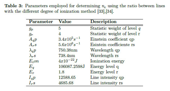
6.4 Electron density using the ratio between lines with the different degree of ionization method
Finding the relation between intensities of this pair of lines from Eq. (31) and (32), the following is obtained:
Where
The population ratio between the states is given by the Saha Equation. In the case of consecutive ionized states, this equation is:
By replacing (32) in (33), the following is obtained
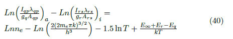
where the subscripts a and i indicate the atomic and ionic variables, respectively. By isolating the density, the following expression is obtained:
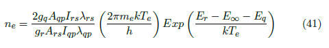
Figure 4(a) presents the lines chosen for the electron density calculation. Values of the variables employed in the corresponding calculation for each pair of lines are given in Table 3.
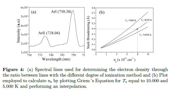
6.5 Electronic density from the stark broadening method
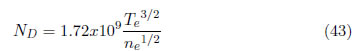
One of the most widely used spectroscopic techniques for determining the electronic density results from the Stark broadening of measured spectral lines. The radiative particles perturbation increase is caused by the electrical fields produced by the environmental electron and ions. In this method, the absolute intensities are not required, only the relative lines shape and width. For densities ne ≥ 1015cm − 3, the broadening is high, and standard spectrometers and monochromators are sufficient. Once the line shapes are determined, the ne value is obtained by comparing the real and theoretical spectral lines width or shape. Details regarding quantum mechanics theory, lines profile shape computation and data tabulations can be found in the text by Griem [43]. The well-isolated Stark line broadening in non-hydrogenic neutral and single ionized atoms (such as lithium and once ionized barium) is dominated by the electronic effect. Then, the full width at half maximum (FWHM) of these lines can be calculated using the electronic impact approximation and corrected by the important ionic quasiestatic broadening; a shift in the line centers (usually toward higher wavelengths) is present far from the normal position. For a good approximation (20 o 30), the medium broadening ∆λ1/2 is given by [44].
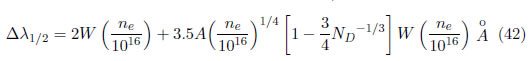
In this expression, the width is measured in Å and the density in cm − 3. The parameter ND represents the number of particles in a Debye sphere and is given by:
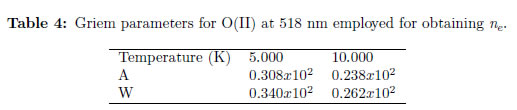
ependent, and they have low fluctuations with respect to the electronic temperature. This formula is applied to lines produced from neutral atoms. To apply this model to single ionized atoms, it is necessary to replace the numeric coefficient 3/4 by 1.2. For all of the lines (different atoms and ions), this expression is useful in the range of ND ≥ 2 and 0.05 < A( ne/1016 )1/4 < 0.5. When ND is less than the given value, the calculation of cuasistatic field, which includes shielding and correlation, are not applicable. When A is outside of the given range, the width and shifting may be determined from the line profile. A list of W (electronic contribution), A (ionic contribution) and D (shifting constant) parameters are given by Griem for several lines of different neutral atoms, from helium to cesium, and single ionized atoms, from lithium to calcium, as shown in [45], [46]. As explained in section 2.3, the total line profile is a combination of different effects. As an example of an experimental application, a study of plasmas generated using a pulsed arc discharge for growing ZnO coatings was performed. To separate the influence of each effect, the instrumental broadening was measured, and a value of 0.1 nm was obtained. Doppler broadening was determined using the Eq. (13), but this value was two orders of magnitude less than the instrumental broadening, which is almost neglecting. To obtain the Stark broadening, Eq. (15) was used with an instrumental broadening of 0.1 nm and a FWHM equal to 0.14 nm, and a value of 0.4 nm was obtained for the Stark broadening. Because the Griem constants are reported by [47] for temperatures of 5.000, 10.000 and 20.000 K, and the experimental temperature is approximately 8100 K, it is necessary to perform an extrapolation. This extrapolation is shown in Figure 4(b). The values employed for creating this figure are presented in Table 4 for the O II (oxygen single ionized) line at 518 nm. With this procedure, we obtained ne on the order of 8 x1012cm − 3.
7 Conclusions
This article has reviewed the progress in experimental research on the characterization of plasmas by determining their physical parameters using optical emission spectroscopy. The advances obtained in this yield have included the development of procedures that enable classical spectroscopic techniques to be applied for plasma diagnostics to the specific cases of sputtering and vacuum arc plasmas. The dependence of the values of the parameters on the experimental conditions is also a characteristic feature of these plasmas, which complicates the comparison of results of different experiments. Nevertheless, significant progress has been achieved in determining accurate values of the plasma electron density, temperature and densities of atoms. However, some important subjects can be mentioned that will require additional effort in research on laser-induced plasma characterization. One of these subjects is the investigation of the formation and evolution of the plasmas through the characterization of their early phase, as near as possible to the laser pulse. The existence of local thermodynamic equilibrium in the plasma is also a relevant topic in this field, which requires the use of accurate measurements of the plasma parameters using different characterization methods. The advantages and applications of the characterization of laser-induced plasmas, particularly the characteristic plasma parameters, are diverse. Knowledge of plasma properties has been used in the selection of experimental conditions for plasma generation and light detection in analytical laser-induced breakdown spectroscopy. In this yield, standard-less analytical procedures have also been developed, which are based on real-time characterization of the plasmas. A promising application of laser-induced plasmas is their use as spectroscopic sources for the measurement of atomic parameters, such as transition probabilities, Stark broadening and shift parameters. In this application, a previous determination of the characteristic plasma parameters, such as temperature and electron density, is necessary. Applications of laser ablation in materials science, such as pulsed laser deposition of thin films, or in chemical analysis, such as inductively coupled plasma methods, have also been improved through the characterization of the plasma formed in the laser ablation process.
References
[1] M. Sharma, B. Saikia, and S. Bujarbarua, ''Optical emission spectroscopy of DC pulsed plasmas used for steel nitriding, Surface and Coatings Technology,'' Surface and Coatings Technology, pp. 203,229–233, 2008.[2] C. Cali, R. Macaluso, and M. Mosca, ''In situ monitoring of pulsed laser indium tin-oxide film deposition by optical emission spectroscopy,'' Spectrochimica Acta Part B: Atomic Spectroscopy, pp. 56, 743-751, 2001.
[3] A. D. Giacomo, V. Shakhatov, and O. D. Pascale, ''Optical emission spectroscopy and modeling of plasma produced by laser ablation of titanium oxides,'' Atomic Spectroscopy, pp. 56, 753-776, 2001.
[4] S. Qin and A. McTeer, ''Plasma characteristics in pulse-mode plasmas using time-delayed, time-resolved Langmuir probe diagnoses,'' Surface and Coatings Technology, p. 6508–6515, 2007.
[5] A. Kono, ''Negative ions in processing plasmas and their effect on the plasma structure,'' Applied Surface Science, p. 115–134, 2002.
[6] C. Seidel, H. Kopf, B. Gotsmann, T. Vieth, H. Fuchs, and K. Reihs, ''A plasma treated and Al metallised polycarbonate: a XPS, mass spectroscopy and SFM study,'' Applied Surface Science, p. 19–33, 1999.
[7] K. Warner and G. M.Hieftje, ''Review: Thomson scattering from analytical plasmas,'' Spectrochimica Acta Part B: Atomic Spectroscopy, p. 201–241, 2002.
[8] T. Duguet, V. Fournée, J. Dubois, and T. Belmonte, ''Study by optical emission spectroscopy of a physical vapour deposition process for the synthesis of complex AlCuFe(B) coatings,'' Surface and Coatings Technology, pp. 9-14, 2010.
[9] N. H. Bings, A. Bogaerts, and J. A. C. Broekaert, ''Atomic Spectroscopy,'' Analytical Chemistry, p. 4317–4347, 2008.
[10] L. H. Allen, Astrophysics: The Atmosphere of the Sun and Stars. The Ronald Press Co, 1963.
[11] M. de Jong and N. Rowlands, ''Proton beam diagnostics using optical spectroscopy, Nuclear Instruments and Methods in Physics Research Section B,'' Beam Interactions with Materials and Atoms, pp. 822-824, 1985.
[12] G. Zambrano, H. Riascos, P. Prieto, E. Restrepo, A. Devia, and C. Rincón, ''Optical emission spectroscopy study of r.f. magnetron sputtering discharge used for multilayers thin film deposition,'' Surface and Coatings Technology, p. 144–149, 2003.
[13] L. García, E. Restrepo, H. Jiménez, H. Castillo, R. Ospina, V. Benavides, and A. Devia, ''Diagnostics of pulsed vacuum arc discharges by optical emission spectroscopy and electrostatic double-probe measurements,'' Vacuum, p. 411–416, 2006.
[14] H. Jiménez, E. Restrepo, and A. Devia, ''Effect of the substrate temperature in ZrN coatings grown by the pulsed arc technique studied by XRD,'' Surface and Coatings Technology, p. 1594–1601, 2006.
[15] Y. M. Kim, J. U. Kim, and J. G. Han, ''Investigation on the pulsed DC plasma nitriding with optical emission spectroscopy,'' Surface and Coatings Technology, p. 227–232, 2002.
[16] H. Chatei, J. Bougdira, M. Remy, and P. Alnot, ''Optical emission diagnostics of permanent and pulsed microwave discharges in H2–CH4–N2 for diamond deposition,'' Surface and Coatings Technology, p. 1233–1237, 1999.
[17] C. Deutsch, ''Validity of complete local thermodynamic equilibrium for hei,'' Physics Letters A, vol. 28, no. 11, pp. 752 - 753, 1969. [Online]. Available: http://www.sciencedirect.com/science/article/pii/0375960169906021
[18] D. Haar, Elements of Statistical Mechanics. Elsevier Science, 1995. [Online]. Available: http://books.google.com.co/books?id=dt8GkhAgd88C
[19] C. Blancard, G. Faussurier, T. Kato, and R. More, ''Effective Boltzmann law and Prigogine theorem of minimum entropy production in highly charged ion plasmas,'' Journal of Quantitative Spectroscopy & Radiative Transfer, p. 75–83, 2006.
[20] J. Aguilera and C. Aragón, ''Multi-element Saha–Boltzmann and Boltzmann plots in laser-induced plasmas,'' Atomic Spectroscopy, p. 378–385, 2007.
[21] E. Garber, ''Some reactions to Planck's law,'' Studies in History and Philosophy of Science, pp. 89-126, 1976.
[22] M. Numano, ''Criteria for local thermodynamic equilibrium distributions of populations of excited atoms in a plasma,'' Journal of Quantitative Spectroscopy & Radiative Transfer, pp. 311-317, 1990.
[23] J. R. J.D. Hey, C.C. Chu, ''Partial local thermal equilibrium in a low temperature hydrogen plasma,'' Journal of Quantitative Spectroscopy & Radiative Transfer, pp. 371-387, 1999.
[24] R. McWhirter, Plasma Diagnostic Techniques. Academic Press, 1965.
[25] C. Aragón and J. Aguilera, ''Characterization of laser induced plasmas by optical emission spectroscopy: A review of experiments and methods,'' Atomic Spectroscopy, p. 893–916, 2008.
[26] G. Cristoforetti, A. D. Giacomo, M. Dell'Aglio, S. Legnaioli, E. Tognoni, V. Palleschi, and N. Omenetto, ''Local Thermodynamic Equilibrium in Laser-Induced Breakdown Spectroscopy: Beyond the McWhirter criterion,'' Atomic Spectroscopy, p. 86–95, 2010.
[27] Q. A. Wang and A. L. Méhauté, ''Nonextensive black-body distribution function and Einstein's coefficients A and B,'' Physics Letters, pp. 301-306, 1998.
[28] L. Cadwell and L. Huwel, ''Time-resolved emission spectroscopy in laser-generated argon plasmas—determination of Stark broadening parameters,'' Journal of Quantitative Spectroscopy & Radiative Transfer, pp. 579-598, 2004.
[29] J. H. Dijkstra and C. D. Vries, ''Differences in natural widths of conversion lines,'' Nuclear Physics, pp. 524-531, 1961.
[30] P. L. Lee, Y. H. Chou, J.-C. Hsieh, and H. K. Chiang, ''An improved spectral width Doppler method for estimating Doppler angles in flows with existence of velocity gradients,'' Ultrasound in Medicine & Biology, pp. 1229-1245, 2006.
[31] V. Milosavljevic, V. Zigman, and S. Djenize, ''Stark width and shift of the neutral argon 425.9 nm spectral line,'' Atomic Spectroscopy, p. 1423– 1429, 2004.
[32] R. Parsons, ''A method for the correction of instrumental broadening of a littrow mount grating spectrometer,'' Infrared Physics & Technology, pp. 197-198, 1968.
[33] V. . N. I. of Standards Technology (NIST). (1999). [Online]. Available: http://www.nist.gov
[34] R. L. Kurucz. (1995) Harvard-Smithsonian Center for Astrophysics. [Online]. Available: http://cfa-www.harvard.edu
[35] J. Zhang, L. Liu, and X. D. T. Ma, ''Rotational temperature of nitrogen glow discharge obtained by optical emission spectroscopy,''Molecular and Biomolecular Spectroscopy, p. 1915–1922, 2002.
[36] J. van Kranendonk, ''Rotational and vibrational energy bands in solid hydrogen,'' Physica, 1959.
[37] J. Koput, S. Carter, and N. C. Handy, ''The vibrational rotational energy levels of silanone,'' Chemical Physics Letters, pp. 1-9, 1999.
[38] Y. Danzaki and K. Wagatsuma, ''Effect of acid concentrations on the excitation temperature for vanadium ionic lines in inductively coupled plasma–optical emission spectrometry,'' Analytica Chimica, p. 171–177, 2001.
[39] H. Park, W. Choe, and S. Yoo, ''Spatially resolved emission using a geometry-dependent system function and its application to excitation temperature pro?le measurement,'' Atomic Spectroscopy, p. 1029–1032, 2010.
[40] D. Vacher, G. Faure, and P. Andre, ''Thermodynamic considerations and optical emission diagnostics of a N2/O2 mixture in an inductively coupled air plasma,'' Atomic Spectroscopy, pp. 309-330, 2001.
[41] A. Sola, M. Calzada, and A. Gamero, ''On the use of the line-to-continuum intensity ratio for determining the electron temperature in a high-pressure argon surface-microwave discharge,'' Journal of Physics, pp. 1099-1110, 1995.
[42] E. Tognoni, A. C. M. Hidalgo, G. Cristoforetti, S. Legnaioli, A. Salvetti, and V. Palleschi, ''Combination of the ionic-to-atomic line intensity ratios from two test elements for the diagnostic of plasma temperature and electron number density in Inductively Coupled Plasma Atomic Emission Spectroscopy,'' Atomic Spectroscopy, p. 435–443, 2007.
[43] H. Griem, ''Stark broadening calculations,'' Journal of Quantitative Spectroscopy & Radiative Transfer, pp. 669-670, 1964.
[44] J. Camacho, L. Díaz, M. Santos, and J. Poyato, ''Time-resolved optical emission spectroscopic measurements of He plasma induced by a high-power CO2 pulsed laser,'' Atomic Spectroscopy, p. 57–66, 2011.
[45] F. Colao, V. Lazic, R. Fantoni, and S. Pershin, ''A comparison of single and double pulse laser-induced breakdown spectroscopy of aluminum samples,'' Atomic Spectroscopy, pp. 1167-1179, 2002.
[46] H. Griem, Spectral line broadening by plasmas. Academic Pres, New York, 1974.
[47] J. Dennaud, A. Howes, E. Poussel, and J.-M. Mermet, ''Study of ionic-to-atomic line intensity ratios for two axial viewing-based inductively coupled plasma atomic emission spectrometers,'' Atomic Spectroscopy, pp. 101-112, 2001.
