DOI: 10.17230/ingciencia.11.22.2

Trajectory Generation from Motion Capture for a Planar Biped Robot in Swing Phase

Generación de trayectorias para un robot bípedo en fase de balanceo a partir de captura de movimiento Humano

Diego A. Bravo M. ¹ and Carlos F. Rengifo R. ²

1 Universidad del Cauca, Popayán, Colombia, dibravo@unicauca.edu.co.

2 Universidad del Cauca, Popayán, Colombia, caferen@unicauca.edu.co.

Received: 29-01-2015 Accepted: 13-04-2015 Online: 31-07-2015

PACS: 87.85.St

Abstract

This paper proposes human motion capture to generate movements for the right leg in swing phase of a biped robot restricted to the sagittal plane. Such movements are defined by time functions representing the desired angular positions for the joints involved. Motion capture performed with a Microsoft Kinect^TM camera and from the data obtained joint trajectories were generated to control the robot's right leg in swing phase. The proposed control law is a hybrid strategy; the first strategy is based on a computed torque control to track reference trajectories, and the second strategy is based on time scaling control ensuring the robot's balance. This work is a preliminary study to generate humanoid robot trajectories from motion capture.

Key words: biped robot; motion capture; trajectory generation; dynamic model

Resumen

En este trabajo se propone la captura de movimiento humano para generar movimientos de la pierna derecha en fase de oscilación de un robot bípedo restringido al plano sagital. Estos movimientos son definidos mediante funciones de tiempo que representan las posiciones angulares deseadas para las articulaciones involucradas. La captura de movimiento realiza con un sensor Kinect^TM y a partir de los datos obtenidos se generaron trayectorias articulares para controlar la pierna derecha del robot en la fase de balanceo. La ley de control propuesta es una estrategia híbrida; la primera estrategia se basa en un control por par calculado para realizar un seguimiento de trayectorias de referencia, y la segunda estrategia se basa en un control por escalado de tiempo para garantizar el equilibrio del robot. Este trabajo es un estudio preliminar para generar trayectorias de robots humanoides a partir de captura de movimiento.

Palabras clave: robot bípedo; captura de movimiento; generación de trayectorias; modelo dinámico

1  Introduction

Nature is a source of inspiration for robotics. The design of bipedal robots is inspired from the functional mobility of the human body, nevertheless, the number of degrees of freedom (DoF), range of motion and speed of an actual biped robot are much more limited compared to humans. The choice of the number of DoF for each articulation is important. The approach consists in analyzing the structure of the robot from three main planes: the sagittal, frontal, and transversal planes. The movement of walking mainly takes place in the sagittal plane; all bipeds have the largest number of important articulations in this plane [1].

Modeling, monitoring, and understanding of human motion based on motion capture is a field of research resurgent during the past decade, with the emergence of applications in sports science, medicine, biomechanics, animation (online games), monitoring and security [2]. Development of these requests is anchored on progress in artificial vision and biomechanics. Although these research areas are often treated separately, the analysis of human movement methodologies requires the integration of computer vision and modeling of the human body as a mechanical system that improves the robustness of this approach [3].

Motion capture is the process of recording a live motion event and translating it into usable mathematical terms by tracking a number of key points in space over time and combining them to obtain a single three-dimensional (3D) representation of the performance; [4]. The subject captured could be anything that exists in the real world and has motion; the key points are the areas that best represent the movement of the subject's different moving parts. These points should be pivot points or connections between rigid parts of the subject. For a human, for example, some of the key points are the joints that act as pivot points and links for the bones. The location of each of these points is identified by one or more sensors, markers, or potentiometers placed on the subject and that serve, in one way or another, as conduits of information to the primary collection device.

Many motion capture systems are available in the market that can be used to acquire the motion characteristics of humans with a relatively high degree of accuracy, for example: PeakMotus (Vicon)^TM SkillSpector^TM and DartFish^TM, among others. These include inertial, optical, and markerless motion capture systems.

Currently, the most common methods for proper 3D capture of human movement require a laboratory environment and setting of markers, sensors accessories body segments. At present, technical progress that has enabled the study of human movement is the measurement of skeletal motion with tags or sensors placed on the skin. The movement of the markers is typically used to derive the underlying relative motion between two adjacent segments to define the motion of a joint accurately. Care of skin movement relative to the underlying bone is the main factor limiting the application of some sensors; [5],[6],[7].

Markerless motion capture systems like Microsoft's Kinect^TM  range camera present alternative new approaches to motion capture technology; [8]. The Kinect^TM  is a light-coded range camera capable of estimating the 3D geometry of the acquired scene at 30 frames per second (fps) with a Depth Sensor with (640 ×480) spatial resolution. Besides its light-coded range camera, the Kinect  also has a color video camera VGA and an array of microphones. The Kinect^TM  has readily been adopted for several other purposes such as robotics; [9], human skeleton tracking [10], and 3D scene reconstruction [11].

Motion capture can be used to allow robots to imitate human motion. Although the motion imitation is merely mapping human motion on to humanoid robots, which have a similar appearance, it is not a trivial problem [12]. The main difficulties to overcome in developing human motion for bipedal robots are the anthropomorphic differences between humans and robots, the physical limits of the robot's actuators, robot balance, [13] and collision avoidance. A control scheme is used to follow the desired trajectories. Two main classes of methods can be used to compute the reference trajectories: either they can be obtained by capturing human motions or computer generated [14]. In this paper, the reference trajectories were obtained from captured human motion data and a hybrid control law strategy allowed a geometrical tracking of these paths.

The hybrid control strategy comprises in a Computed Torque Control (CTC) and time scaling control; this control strategy switches according to the desired Zero Moment Point (ZMP). The approach ensured the balance of the biped robot within safety limits. The control law with time-scaling is defined in such a way that only the geometric evolution of the biped robot is controlled, not the temporal evolution. The concept of control with time-scaling was introduced by Hollerbach [15] to track the reference trajectories in a manipulator robot. It has also been implemented to control mechatronics systems, [16]. In [17], Chevallereau applied the time scaling control of the underactuated biped robot without feet and actuated ankles. This work sought to define the sequence of joint movements that allow a biped robot to make the swing phase of the right leg similar to that of humans by using motion capture data, the proposed control law will be validated in a planar biped robot with feet and actuated ankles.

The rest of the paper is structured as follows: section 2 shows the dynamic model of the robot; section 5 calculates the control law, followed by its results in section 6 and concluding the paper in section 7.

2  Dynamic model of the robot

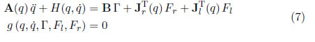
The dynamical model was derived from the biped robot Hidroïd, [18] which include the dynamic parameters to calculate the inertia matrix and vector of forces. The Lagrangian representation of the robot's dynamic model is the following:

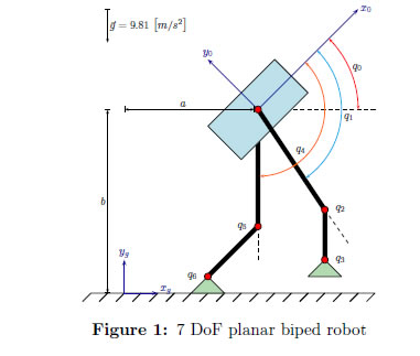
In the previous model q ⁹ is the vector of generalized coordinates. This vector contains three types of coordinates: (i) (x₀,y₀) denoting the Cartesian position of the reference frame < x₀,y₀ > in the reference frame < x_g,y_g > , (ii) q₀ denoting the orientation of the reference frame < x₀,y₀ > with respect to the reference frame < x_g,y_g > , (iii) (q₁,...,q₆) denoting the six joint positions depicted in Figure 1.

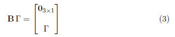
Vectors ⁹ and ⁹ are respectively the first and second derivatives of q with respect to time. ^9×9 is the robot's inertia matrix. H ⁹ is the vector of centrifugal, gravitational, and Coriolis forces. Matrix ^9x6 contains only ones and zeros. The first three rows of are zero, indicating that Γ has no direct influence on the acceleration of the first three generalized coordinates. The following 6 rows of B form an identity matrix, indicating that Γ_i (i = 1, ... , 6) directly affects i... ¸ ⁶ is the vector of torques applied to the joints of the robot. This leads to fulfilling the following property:

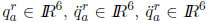
r ^3×9 is the jacobian matrix relating the linear and angular velocities of the robot's right foot in the reference frame < x_g, y_g > with the vector

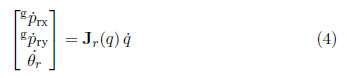
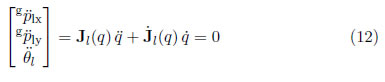
In (4), are the linear velocities of the reference frame < x₃, y₃ > with respect to < x_g, y_g >, whereas that, is the angular velocity of the reference frame < x₃, y₃ > with respect to < x_g, y_g >. The matrix _l ^3×9 is used to express the linear and angular velocities of the robot's left foot to the ground, (Figure 2).

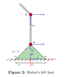
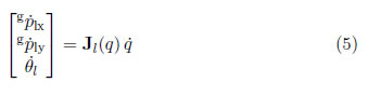
In (5), are the linear velocities of the reference frame < x₆, y₆ > with respect to < xg, yg >, whereas that, is the angular velocity of the reference frame < x₆, y₆ > with respect to < x_g, y_g >. The unknowns of the previous model are ⁹, F_r ³ and F_l ³. That is; there are 9 equations and 15 variables. The required additional equations can be obtained by using complementarity conditions related to normal and tangential foot reaction forces [19]. However, as it was demonstrated by several authors complementarity conditions can be written as an implicit algebraic equation [20],[21]:

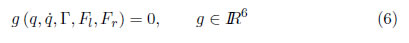
The unknowns in (6) are F_r and F_l. In summary, the robot's dynamic behaviour is described by the differential equation (1) subject to the algebraic constraint (6)

Model (1) allows to represent robot's dynamic behavior in all phases of a gait pattern: single support on left foot, double support and single support on the right foot. In the following, (7) will be called the simulation model, and it will be used to validate the proposed control strategy. To design of such strategy is also necessary another model called synthesis control model. This latter model depends on the phase of the gait pattern. In most cases three different models are used, one of them for each phase of the gait pattern. As the proposed control strategy for motion imitation will be tested when robot is resting on the left foot and right limb is trying to track a joint reference motion obtained by a Kinect system, only the synthesis control model for single support phase on the left foot will be required.

3 Reference motion

The six joint angle trajectories, denoted as (i = 1, ... , 6), are estimated from N + 1 Cartesian positions measured by a motion capture system based on Microsoft's Kinect ^TM camera. The trajectory for the joint i is represented by using a set of N third order polynomials called cubic splines,

c_0,j,i, c_1,j,i, c_2,j,i, c_3,j,i are the coefficients of a third order polynomial describing the reference motion of the joint i in the time interval t [t_j−1, t_j] (j = 1 ...N + 1). The length of each time interval is constant and equal to the sampling time used by the motion capture system (h = t_j − t_j−1).

4 Control for the single support phase on the left foot

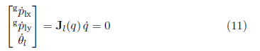
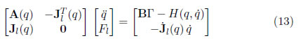
When the robot is resting on the left foot, the model (1) can be rewritten as:

The unknowns of the previous model are ⁹ and F_l 3. That is; there are 9 equations and 12 variables. For the purpose of the synthesis of the control system only, the previous model will be considered as subject to immobility constraints on the left foot immobility

In order to involve the unknowns of the problem in the three equations above, these are derived twice with respect to time. By deriving once, we obtain:

By deriving once again:

By combining equations (9) and (12) a model relating and F_l as a function of q, and Γ is obtained

rewriting the constraint (12) in the form:

With q_u being the vector containing the undriven coordinates and q_a the driven coordinate vector

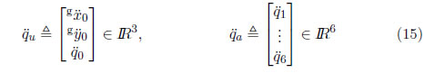
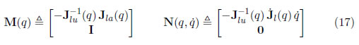
Matrix _lu(q) ^3×3 is composed by the first three columns of _l(q) and _la(q) ^3×6 by the last six columns. By solving _u of (14) we obtained:

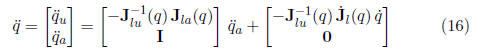
Equation indicates that the contact between the left foot and the ground leads to the acceleration of the coordinates not being directly driven by the acceleration of the coordinates actuated. In order to lighten the mathematical notation, the following variables are defined:

In the following the arguments of , , and will be omitted. Substituting = a + in the dynamic model (9)

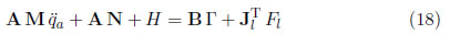
Equation (18) is multiplied by and by simplifying we obtain

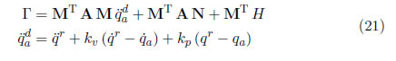
If _a is replaced by the desired acceleration and it is calculated as follows, equation (19) becomes a classical computed torque control [22]

being the joint reference motion obtained by using the motion capture system. By replacing in (19) we obtain the following equations which allow to calculate the joint torques required to the joint coordinates follow theirs respective reference values

5 Hybrid control

Control law (21) ensures the convergence of the joint variables q_i(t), _i(t) and _i(t) (i = 1 ... 6) towards the reference motion and described in section 3. However, tracking of these variables does not prevent the robot may fall. To prevent falling, a technique called time-scaling, initially developed for robot manipulators [15], was used applied in [17] to control of the Zero Moment Point [13] (ZMP) of a bipedal robot. This technique, unfortunately, requires to know the desired position of the ZMP, which cannot be obtained by our Kinect-based motion capture system. This reason has motivated us to propose a new control strategy using a rule based on the following variables: (i) the current position of the robot's ZMP, denoted px and (ii) the length of the foot, denoted lf :

If p_x, satisfies the condition p_x ≤ 0.45 l_f ,

then the control law (21) is used. Other

wise set the desired position of the ZMP,

denoted = 0.45 sign(p_x) l_f , and apply

time-scaling control.

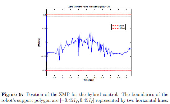
The upper limit of the inequality in the paragraph above ensures that the ZMP never reaches the edges of the foot. In this way, the ZMP belongs in the interval [-0.45 l_f , 0.45 l_f ] and the proposed control law allows track a desired reference motion and maintain robot's equilibrium without requiring to know the ZMP of the performer (a human being).

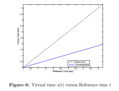
To apply time-scaling control, the reference trajectory (8) must to be parametrized as a function of a variable s(t) called virtual time

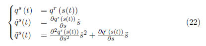
Given s(t), a unique trajectory is defined. Any trajectory defined by (22) corresponds to the same path in the joint space as the reference trajectory, but the evolution of the robot with respect to time may differ. If instead of q_r(t), ^r(t) and ^r(t), the variables defined by (22) are used to calculate , (21) becomes

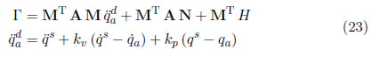
With s = t, = 1 and = 0, the control law (23) is a classical CTC, otherwise, it is a time scaling control. The procedure to find is explained in the next section.

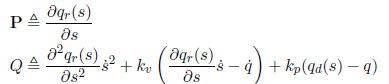
5.1 Dynamics of for a given desired ZMP position

Model (9) can be rewritten as:

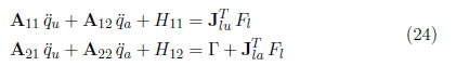
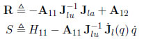
Here, A₁₁ ^3x3, A₁₂ ^3x6, H₁₁ ^3x1, F_l ^3x1, A₁₂ ^6x3, A₂₂ ^6x6, H₁₂ ^6x1 and Γ ^6x1. _u can be expressed as function of _a by using (14). By using (22), _a may in turn be rewritten as:

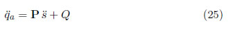
with

By combining (14) and (25), the first row of (24) becomes:

with

Expression (26) contains 3 equations and 4 unknowns ( and F_l ³). The additional equation allowing to fix the ZMP position will be presented in the next section.

5.2 Dynamic of zero moment point.

The concept of Zero Moment Point (ZMP) was first introduced by Vukobratovic [13], is used for the control of humanoid robots. The ZMP specifies the point where the reaction forces generated by the foot contact with the ground produce no moment in the plane of contact, it is assumed that the surface of the foot is flat and has a coefficient of friction sufficient to prevent slippage. The zero moment point (ZMP) can be calculated as follows:

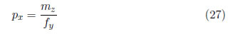
P_x being the zero moment point, m_z the angular momentum on axis z and f_y the reaction force of the ground exerted on foot. In an equivalent way, if is the desired position for the ZMP, such value have to satisfy

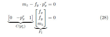
When (28) is combined with (26), the resulting system has four equations and four unknowns

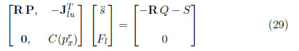
The question is: ¿how to select if the ZMP of the performer is not known?

5.3 Summary of the hybrid strategy

If p_x ≤ 0.45 lf , then Γ is calculated by using (21) and is set to zero. Otherwise, = 0.45 sign(px) lf , use (29) to compute and (23) to obtain Γ.

6 Results and discussion

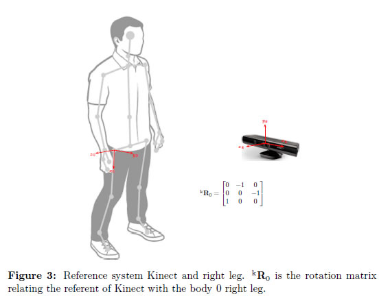
We can represent human anatomy as a sequence of rigid bodies (links) connected by joints; [3]. Kinect ^TM allows optical tracking of a human skeleton and gives the Cartesian coordinates (x, y, z) of 20 joint points. In our case, we are interested in joint coordinates of the lower limbs in the sagittal plane. So, it was necessary to develop an application to transform Cartesian coordinates (x, y, z) into joint coordinates (q₁, ... , q₆) by using inverse kinematics. The experiment was designed to capture motion data of the right leg, consisting of moving the right leg in swing phase while the left leg remains still. The reference trajectories for swing phase of the right leg were obtained through a Microsoft's Kinect ^TM camera at 30 fps. In this experiment the user is in front of Kinect, the rotation matrix that relates the referent of Kinect with the body 0 right leg, is writes:

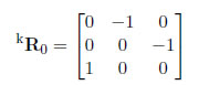
The sensor position and the reference axes shown in Figure 3. The reference trajectories of the joint positions are described as a function of time q^r(t).

The results shown in Figure 4 are relative to measurements of kinematic variables for the movement of a walking male of a height of 1.65m. The sinusoidal feature of the movement of the hip articulation q₁ is easy to identify. The shapes of the trajectory for the hip q₁ and right knee q₂ are similar to those reported in the literature for the swing phase [23],[24]. The trajectory q₃ represents the angular motion of the heel in a sagittal plane, the rapid variation is by poor detection of anatomical landmarks during the toe-off and ground contact phases of movement, which is likely due to the inability of the machine learning algorithm to accurately identify landmarks in this position when compared to regular standing positions, and the failure to identify multiple significant land marks on the foot such as the metatarsophalangeal and calcaneus, which would allow for more precise detection of gait events, [25]. Figure 5 shows a geometrical tracking, rather than temporal tracking of the reference trajectory.

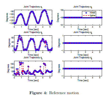
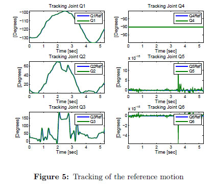
Figure 4 shows the joint trajectories for lower limb data taken from human motion capture in the swing phase at a frequency of 30 fps and trajectories filtered with . Cubic spline interpolation was used between each of the joint positions to ensure the continuity of the paths. The primary articulations associated with human locomotion are those of the hips, the knees, the ankles and the metatarsal articulations. Hip movement combined with pelvis rotation enables humans to lengthen theirsstep, [1]. During a walking cycle, the movement of the hip in the sagittal plane is essentially sinusoidal. Thus, the thigh moves from back to front and vice versa. The articulation of the knee allows for flexion and extension movements of the leg during locomotion. As for the ankle, flexion movements occur when the heel is re-grounded. There is a second flexion during the balancing phase.

Due to the robot cannot execute the motion with all constraints satisfied, then the robot moves slower in this region of the curve, like Figure 6, where the slope of the curve that represents the virtual time is always less than one.

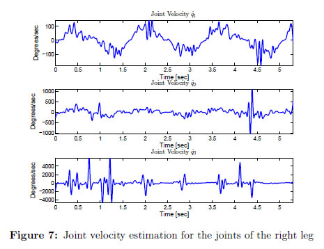
To implement the control law (23), velocity, and joint acceleration measurements are necessary. Because the velocity and acceleration are not directly measurable on the paths obtained by Kinect, these are calculated from measurements of joint position. To estimate the velocity and acceleration, first the interpolation between each joint position is performed by using third order polynomials. Then, the resulting sequence of polynomials is derived for the first time to estimate the speed and the second time to calculate acceleration. The joint velocity of the right leg in swing phase is shown in Figure 7. For these reasons, values of desired joint coordinates q^r(t), r(t) and r(t) were calculated offline. Unfortunately, Kinect is sensitive to infrared light, this generates a high level of noise in the measurements, despite being filtered, [26]. However, studies have been conducted to improve its accuracy by implementing a Kalman filter in human gait studies, [27]. Although this approach was not used in the development of this work.

The controller switches between two control laws to achieve a stable result. When the constraint p_x ≤ 0.45 l_f is met, the control law is a classic CTC, where = 0. Here, the controller is tuned for a settling time of 0.1 seconds and damping factor of 0.707. On the other hand, the time scaling control is used to ensure the stability of the robot and fulfill the constraint p_x ≤ 0.45 l_f . Then, the controller is tuned for a settling time of 0.01 seconds and damping factor of 1. The simulation of the whole system was done in the MATLAB Simulink © programming environment.

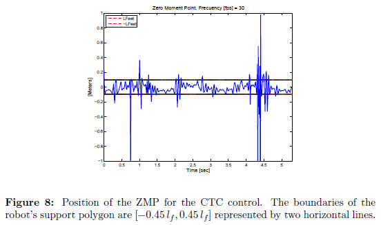
For the classic CTC control, the temporal evolution of the ZMP is shown in Figure 8. Although the robot makes tracking reference trajectories, the ZMP leaves the limits of the support polygon, rendering the system unstable. This case may be dangerous. We propose conducting time scaling control when this situation occurs.

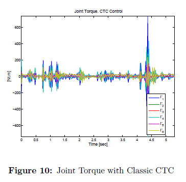
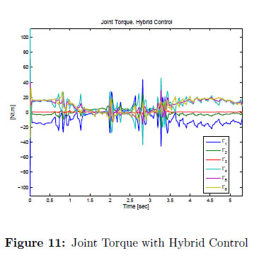
In Figure 9, at time t = 0 second, the ZMP trajectory reaches the upper limit of the support polygon. Then, time scaling control is activated to ensure the ZMP remains within the support polygon for the motion and provide the robot's stability. Vector Γ ⁶ for each one of joints (q₁, q₂, ... , q₆) is a plot. Figure 10 shows the input torques for classic CTC control. The values of Γ₁, Γ₂, Γ₃ are of the joints of left leg, whereas Γ₄, Γ₅, Γ₆ are of the joints of right leg. The values are big, in average 200 [Nt . m] making the control law impracticable. But, for the hybrid control the average is 40 [Nt ^. m] decreasing in a relationship (1 : 5), see Figure 11. This law control is practicable, considering that the total mass of the robot for the simulation is 45.75 [Kg] or a weight of 448.82 [Nt].

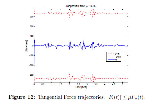
The constraint p_x ≤ 0.45 l_f is only satisfied by using the hybrid control. Figure 12 shows that the tangential force is within the limits of the cone of friction for friction coefficient μ = 0.75. Therefore, the robot could not slide and fall.

7 Conclusion

The trajectory generation from motion capture for a planar biped robot in swing phase is presented. The robot modeled is a planar biped with only six actuators and underactuated during the single support phases. The reference trajectory to be tracked using the proposed hybrid control strategy was calculated off-line via human motion capture. The simulations show that the hybrid control strategy of joint trajectories ensures only geometrical tracking of the reference trajectory, besides the robot's stability.

The comparison between the control techniques, classic CTC and time scaling control, show that although both methods allow tracking reference trajectories, only the hybrid control ensures robot stability, but not tracking of time references. This is an open problem, to be solved: tracking reference trajectories in space and time to provide robot stability.

In our future work, we will experimentally validate the hybrid control strategy with the humanoid robot Bioloid ^TM by means of trajectories obtained from human motion capture and analyze stability for trajectory generation of a biped robot from human motion capture.

Acknowledgments

The authors would like to recognize and express their sincere gratitude to Universidad del Cauca (Colombia) for the financial support granted during this project.

References

[1] C. Chevallerau, G. Bessonnet, G. Abba, and Y. Aoustin, Bipedal Robots. Modeling, design and building walking robots, 1st ed. Wiley, 2009.         [ Links ] 26, 40

[2] B. Rosenhahn, R. Klette, and D. Metaxas, Human Motion: Understanding, Modelling, Capture, and Animation. Springer, 2008.         [ Links ] 26

[3] K. Abdel-Malek and J. Arora, Human Motion Simulation: Predictive Dynamics. Elsevier Science, 2013.         [ Links ] 27, 37

[4] A. Menache, Understanding motion capture for computer animation, 2nd ed. Elsevier, 2011.         [ Links ] 27

[5] A. Cappozzo, A. Cappello, U. Croce, and F. Pensalfini, "Surface-marker cluster design criteria for 3-d bone movement reconstruction," Biomedical Engineering, IEEE Transactions on, vol. 44, no. 12, pp. 1165-1174, Dec 1997.         [ Links ] [Online]. Available: http://dx.doi.org/110.1109/10.649988 27

[6] J. P. Holden, J. A. Orsini, K. L. Siegel, T. M. Kepple, L. H. Gerber, and S. J. Stanhope, "Surface movement errors in shank kinematics and knee kinetics during gait," Gait & Posture, vol. 5, no. 3, pp. 217 227, 1997.         [ Links ] 27

[7] C. Reinschmidt, A. van den Bogert, B. Nigg, A. Lundberg, and N. Murphy, "Effect of skin movement on the analysis of skeletal knee joint motion during running," Journal of Biomechanics, vol. 30, pp. 729-732, 1997.         [ Links ] 27

[8] C. D. Mutto, P. Zanuttigh, and G. M. Cortelazzo, Time-of-Flight Cameras and Microsoft Kinect(TM). Springer Publishing Company, Incorporated, 2012.         [ Links ] 27

[9] G. Du, P. Zhang, J. Mai, and Z. Li, "Markerless kinect-based hand tracking for robot teleoperation," International Journal of Advanced Robotic Systems, vol. 9, no. 10, 2012.         [ Links ] 28

[10] L. A. Schwarz, A. Mkhitaryan, D. Mateus, and N. Navab, "Human skeleton tracking from depth data using geodesic distances and optical flow," Image and Vision Computing, vol. 30, no. 3, pp. 217 226, 2012.         [ Links ] 28

[11] S. Izadi, D. Kim, O. Hilliges, D. Molyneaux, R. Newcombe, P. Kohli, J. Shotton, S. Hodges, D. Freeman, A. Davison, and A. Fitzgibbon, "Kinect-fusion: Real-time 3d reconstruction and interaction using a moving depth camera," in Proceedings of the 24th Annual ACM Symposium on User Interface Software and Technology, ser. UIST '11. New York, NY, USA: ACM, 2011, pp. 559-568.         [ Links ] 28

[12] K. Munirathinam, S. Sakkay, and C. Chevallereau, "Dynamic motion imitation of two articulated systems using nonlinear time scaling of joint trajectories," in International Conference on Intelligent Robots and Systems (IROS), Algarve, Portugal, May-June 2012.         [ Links ] 28

[13] M. Vukobratovié, "Zero-moment point. thirty five years of its life," International Journal of Humanoid Robotics, vol. 01, no. 01, pp. 157-173, 2004.         [ Links ] 28, 34, 36

[14] S. Kajita and B. Espiau, "Legged robots," in Springer Handbook of Robotics, B. Siciliano and O. Khatib, Eds. Springer Berlin Heidelberg, 2008, pp. 361-389.         [ Links ] 28

[15] J. M. Hollerbach, "Dynamic scaling of manipulator trajectories," in American Control Conference, 1983, 1983, pp. 752-756. 28, 34 Ed. InTech, 2008, ch. 22.         [ Links ] 28

[17] C. Chevallereau, "Time-scaling control for an underactuated biped robot," IEEE Transactions on Robotics and Automation, vol. 19, no. 2, pp. 362 368, 2003.         [ Links ] 28, 34

[18] S. Alfayad, "Robot humanoïde hydroïd: Actionnement, structure cinématique et stratègie de contrôle," Ph.D. dissertation, Université de Versailles Saint Quentin en Yvelines, 2009.         [ Links ] 29

[19] C. Rengifo, Y. Aoustin, F. Plestan, and C. Chevallereau, "Contac forces computation in a 3D bipedal robot using constrained-based and penalty-based approaches," in International Conference on Multibody Dynamics, Brusselles, Belgium, 2011.         [ Links ] 31

[20] C. Kanzow and H. Kleinmichel, "A new class of semismooth newton-type methods for nonlinear complementarity problems," Computational Optimization and Applications, vol. 11, no. 3, pp. 227 - 251, December 1998.         [ Links ] 31

[21] M. C. Ferris, C. Kanzow, and T. S. Munson, "Feasible descent algorithms for mixed complementarity problems," Mathematical Programming, vol. 86, no. 3, pp. 475-497, 1999.         [ Links ] 31

[22] W. Khalil and E. Dombre, Modeling, Identification and Control of Robots, 2nd ed., ser. Kogan Page Science. Paris, France: Butterworth Heinemann, 2004.         [ Links ] 34

[23] S. N. Whittlesey, R. E. van Emmerik, and J. Hamill, "The swing phase of human walking is not a passive movement," Motor Control, vol. 4, no. 3, pp. 273-292, 2000.         [ Links ] 38

[24] T. Flash, Y. Meirovitch, and A. Barliya, "Models of human movement: Trajectory planning and inverse kinematics studies," Robotics and Autonomous Systems, vol. 61, no. 4, pp. 330 - 339, 2013.         [ Links ] 38

[25] R. A. Clark, Y.-H. Pua, K. Fortin, C. Ritchie, K. E. Webster, L. Denehy, and A. L. Bryant, "Validity of the microsoft kinect for assessment of postural control," Gait & Posture, vol. 36, no. 3, pp. 372 - 377, 2012.         [ Links ] 38

[26] D. Webster and O. Celik, "Experimental evaluation of microsoft kinect's accuracy and capture rate for stroke rehabilitation applications," in Haptics Symposium (HAPTICS), 2014 IEEE, Feb 2014, pp. 455-460.         [ Links ] 41

[27] B. Sun, X. Liu, X.Wu, and H.Wang, "Human gait modeling and gait analysis based on kinect," in Robotics and Automation (ICRA), 2014 IEEE International Conference on, June 2014, pp. 3173-3178.         [ Links ] 41