


Services on Demand
Journal
Article
 English (pdf)
 Article in xml format
 Article references
 Send this article by e-mail
Indicators
-
 Cited by SciELO
 -
 Access statistics
Related links
-
 Cited by Google
 -
 Similars in
SciELO
Similars in
SciELO -
 Similars in Google
Share

 Permalink
Ingeniería y Ciencia
Print version ISSN 1794-9165
ing.cienc. vol.11 no.22 Medellín July/Dec. 2015
https://doi.org/10.17230/ingciencia.11.22.4
ARTÍCULO ORIGINAL
DOI: 10.17230/ingciencia.11.22.4
Efficient Software Implementation of the Nearly Optimal Sparse Fast Fourier Transform for the Noisy Case
Implementación software eficiente de la Transformada de Fourier Escasa casi óptima para el caso con ruido
Alexander López-Parrado 1 and Jaime Velasco Medina 2
1 Universidad del Quindío, Armenia, Quindío, Colombia, parrado@uniquindio.edu.co
2 Universidad del Valle, Cali, Valle, Colombia, jaime.velasco@correounivalle.edu.co.
Received: 06-04-2015 Accepted: 02-07-2015 Online: 31-07-2015
MSC: 65T50, 68W20, 68W25 PACS: 02.30.Nw, 33.20.Ea, 89.20.Ff
Abstract
In this paper we present an optimized software implementation (sFFT-4.0) of the recently developed Nearly Optimal Sparse Fast Fourier Transform (sFFT) algorithm for the noisy case. First, we developed a modified version of the Nearly Optimal sFFT algorithm for the noisy case, this modified algorithm solves the accuracy issues of the original version by modifying the flat window and the procedures; and second, we implemented the modified algorithm on a multicore platform composed of eight cores. The experimental results on the cluster indicate that the developed implementation is faster than direct calculation using FFTW library under certain conditions of sparseness and signal size, and it improves the execution times of previous implementations like sFFT-2.0. To the best knowledge of the authors, the developed implementation is the first one of the Nearly Optimal sFFT algorithm for the noisy case.
Key words: Sparse Fourier Transform; multicore programming; computer cluster.
Resumen
En este artículo se presenta una implementación software optimizada (sFFT-4.0) del algoritmo Transformada Rápida de Fourier Escasa (sFFT) Casi Óptimo para el caso con ruido. En primer lugar, se desarrolló una versión modificada del algoritmo sFFT Casi Óptimo para el caso con ruido, esta modificación resuelve los problemas de exactitud de la versión origial al modificar la ventana plana y los procedimientos; y en segundo lugar, se implementó el algoritmo modificado en una plataforma multinúcleo compuesta de ocho núcleos. Los resultados experimentales en el agrupamiento de computadores muestran que la implementación desarrollada es más rápida que el cálculo directo usando la biblioteca FFTW bajo ciertas condiciones de escasés y tamaño de señal, y mejora los tiempos de ejecución de implementaciones previas como sFFT-2.0. Al mejor conocimiento de los autores, la implementación desarrollada es la primera del algoritmo sFFT Casi Óptimo para el caso con ruido.
Palabras clave: Transformada de Fourier Escasa; programación multi núcleo; agrupamiento de computadoras.
1 Introduction
The sFFT term refers to a family of algorithms which allow the estimation of the Discrete Fourier Transform (DFT) of a sparse signal, faster than the FFT algorithms found in the literature [1],[2],[3],[4]; in this case, it is assumed that the signal is sparse or approximately sparse in the DFT domain.
In the one hand, researchers from the Massachusetts Institute of Technology (MIT) presented two sFFT algorithms [2] which improve the runtime over all the previous developments [1],[5],[6],[7] including the most optimized conventional FFT algorithms like FFTW [8]; the first algorithm is intended for the noiseless case, and the second algorithm is intended for the noisy case.
On the other hand, to the best of our knowledge there are only four software implementations of the MIT sFFT algorithms reported in literature; the first one was developed by the algorithm authors for the first version of the sFFT algorithm [1]; the second one is an optimized implementation of the first version of the sFFT algorithm [9]; the third one is a GPU-based implementation of the first version of the sFFT algorithm [10]; and the fourth one is an optimized implementation of the Nearly Optimal sFFT algorithm for the noiseless case [11]. Therefore, there is no software implementation reported in literature of the Nearly Optimal sFFT algorithm for the noisy case, which is of practical interest for scientific researchers.
Therefore considering the above, the main contribution of this paper is the development of a modified version of the Nearly Optimal sFFT algorithm and its optimized software implementation on a multicore environment provided by a Beowulf cluster. The modified algorithm has an improved accuracy when compared with the original version described in [2], by modifying the flat window and the procedures; to the best of our knowledge, the modified algorithm is the first implementation of the Nearly Optimal sFFT algorithm for the noisy case, and it is very suitable for hardware implementation using ASICs or FPGAs.
The rest of the paper is organized as follows: Section 2 describes the Nearly Optimal sFFT algorithm, section 3 presents the modified version of the Nearly Optimal sFFT algorithm, section 4 presents experimental results, and section 5 presents the conclusions and future work.
2 Nearly optimal Sparse Fast Fourier Transform algorithm
In this section, we initially present some concepts about sFFT, then we describe the Nearly Optimal sFFT algorithm, and finally we show some software simulations to verify the basic concepts. Given a discrete time signal x 
 of length N, its N-point Discrete Fourier Transform (DFT)
  is defined in Eq. 1.
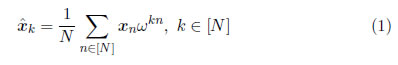
Where N is a power of two, [N] denotes the set of indexes {0,1,…,N−1 }, and ω = e−i 2 π/ N is the N-th root of unity. In this case, the number of non-zero elements of the vector is named the sparsity order K and it is defined in Eq. 2.
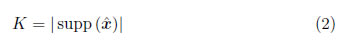
Where supp() is the set of indexes of the non-zero elements of the vector . Then, a time domain signal x is sparse in the DFT domain if K << N.
In this context, a set of algorithms named sFFT takes advantage of the signal sparsity in the DFT domain to speed up the runtime of the Fast Fourier Transform (FFT) algorithms used to calculate the DFT [1],[2],[3]. Then, taking into account the above, we performed the software implementation of the Nearly Optimal sFFT algorithm for the noisy case presented in [2] by considering the mathematical tools: pseudo-random spectral permutation [1],[7], flat filtering window [2] and hashing function [1],[2]; and using the procedures for approximate sparse recovery [6],[2] and median estimation [1],[2],[7].
2.1 Mathematical background about sFFT
2.1.1 Pseudo-random spectral permutation
This permutation isolates spectral components from each other [7], and it is performed as described in Eq. 3.

Where xp and p are the permuted spectrum signals in time domain and DFT domain, respectively; πp(k,σ,N) = σk mod N is the spectral permutation function; and σ {2c+1 | c [N/2]} and a [N] are the spectral permutation parameters. The spectral permutation function translates the frequency bin from the k-th location to the πp(k,σ,N)-th location, in this case σ−1 mod N exists for all odd σ if N is a power of two. The sFFT algorithm chooses at random the spectral permutation parameters σ and a from a uniform distribution, then the spectral permutation with these pseudo-random parameters is related to a pseudo-random sampling scheme [1],[7].
2.1.2 Flat filtering window
The flat window is a mathematical tool that allows to reduce the FFT size from N to B points, this is accomplished by extending a flat passband region of width N/B around each sparse component; this approach replaces the filter bank of previous sFFT algorithms [7],[5]; additionally, the flat window avoids the use of non equispaced data FFTs [12]. A flat window is defined with the time domain vector G  and the DFT domain approximation
  [1], and the work in [2] presents a flat window with the parameters B ≥ 1, δ > 0, α > 0, |\operatornamesupp(G)|=O(B/αlog(N/δ)), where the conditions described in Eq. 4 are satisfied [2].
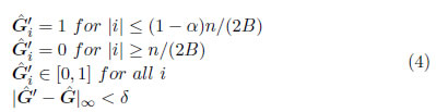
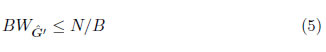
It is important to mention that the practical construction of a flat window lead to a total bandwidth  in the DFT domain that satisfies Eq. 5.
Finally, the windowing process is described in Eq. 6, and it is performed in time domain after the pseudo-random spectral permutation is carried out.
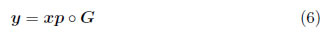
Where y is the windowed signal in time domain.
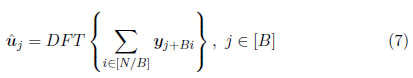
2.1.3 Hashing function The hashing function obtains B points from the N-point spectrum of the signal y, these points are separated by N/B bins where B is a power of two, and they are obtained by calculating the B-point DFT of the sub-sampled signal y. The vector that has the hashes of the signal y is 
 and it is calculated using Eq. 7, [1],[2].
From Eqs. 4, 6 and 7, it is possible to note that for each sparse component of the signal x there is one hash located in the offset given by Eq. 8

Where hr(j,σ,N,B)=  is the round-hash function; and hr(j,σ,N,B) mod B is the index of an element of the vector that hashes a single sparse component. It is important to note, that due to the condition presented in Eq. 5, the hash can be zero which could reduce the capability of the sFFT algorithm to locate a sparse component.
Also, it has been noted that the use of pseudo-random spectral permutation and small support windows leads to a sub-Nyquist random sampling scheme; where, under certain conditions, the average sampling rate is below Nyquist.
2.2 Procedures and sFFT algorithm description
The sFFT algorithm, presented in [2] and described in Alg. 1, calculates the DFT estimation  of a noisy sparse signal; the algorithm has the following input parameters: the time domain signal x, the sparsity order K, the constant ϵ for the maximum error in the sparse recovery, and the parameter δ of the flat window [2].
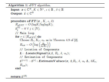
The sFFT algorithm calculates the DFT of a noisy sparse signal using four processing stages: the first one adjusts the flat window parameters Br, αr, and Kr; the second one locates the sparse components using the procedure LocateSignal; the third one estimates the DFT values of the located sparse components using the procedure EstimateValues; and the fourth one updates the DFT estimation by accumulating the results of the procedure EstimateValues. In this case, the above procedures use the procedure HashToBins.
2.2.1 Procedure HashToBins This procedure, presented in Alg. 2, calculates the hashes-error by subtracting the hashes of from the hashes , and it has the following input parameters: the time domain signal x; the instantaneous estimation of ; the parameter B; the spectral permutation parameters σ, and a; and the flat window parameters δ, and α.
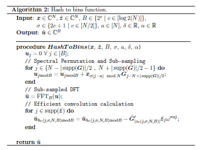
This procedure calculates the hashes-error using three processing stages: the first one simultaneously calculates in time domain the pseudo-random spectral permutation, the windowing, and the hashing process; the second one calculates the DFT domain hashes by performing the B-point FFT of the time domain hashes u; and the third one calculates the hashes-error by subtracting the DFT domain hashes of from the hashes [2].
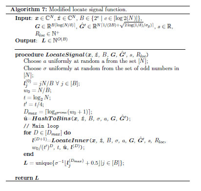
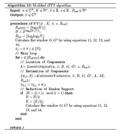
2.2.2 Procedure LocateSignal This procedure, presented in Alg. 3, calculates the set L  O(B) of frequency bins corresponding to O(B) sparse components found in x; and it has the following input parameters: the time domain signal x; the instantaneous estimation of ; the parameter B; and the flat window parameters δ, and α.
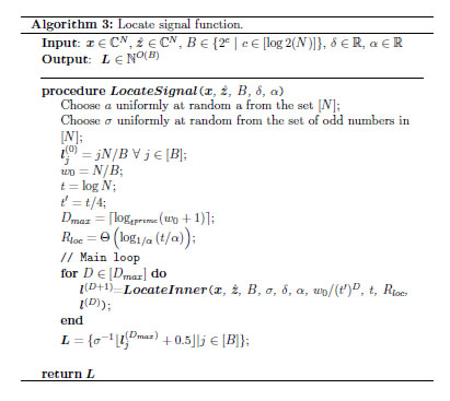
This procedure locates the sparse components of x using four processing stages: the first one sets the initial conditions, the second one adjusts the frequency locations, the third one reduces the search region, and the fourth one inverts the spectral permutation. The setting of initial conditions is performed by pre-calculating an initial guess of value lj(0)=jN/B ∀ j [B] of frequency locations in the permuted spectrum, and by pre-calculating the initial values of w, t, Dmax, and Rloc, where w is the width of the region for searching the frequency adjustment, t is the number of candidate adjustments in w, Dmax is the number of adjustments, and Rloc is the number of location iterations for each adjustment. The adjustment of frequency locations is performed by using Dmax times the procedure LocateInner. The reduction of search region is performed by dividing w by a factor 1/(t′)D−1 at the D-th adjustment, this reduction allows a systematic refining of the frequency location. Finally, the spectral permutation inversion is performed by calculating the function πp−1(k,σ,N) on each located frequency.
2.2.3 Procedure LocateInner This procedure, presented in Alg. 4, performs the adjustment of the frequency locations in the permuted spectrum as described in [2], and it has the following input parameters: the time domain signal x; the instantaneous estimation of ; the parameter B; the spectral permutation parameter σ, the flat window parameters δ, and α; the width of search region w; the number of candidate adjustments t; the number of location iterations Rloc; and the current estimation of frequency locations l.
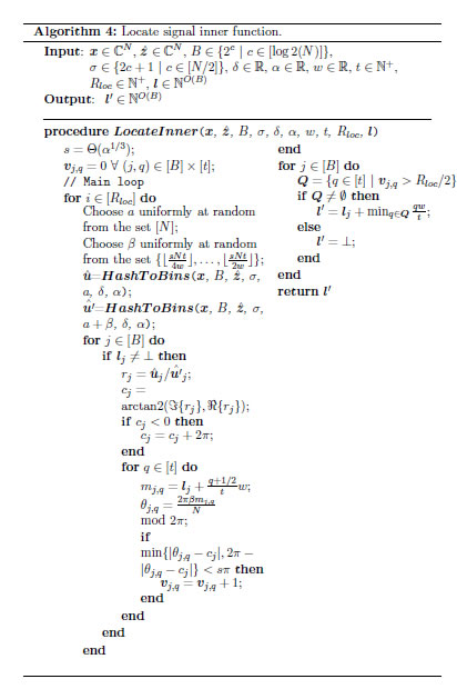
This procedure performs the adjustment of the frequency location using five processing stages: the first one sets the initial conditions, the second one calculates the hashes-error, the third one calculates the angles of the hashes-error and candidate frequency bins, the fourth one performs the voting stage, and the fifth one locates the frequency bins. The setting of initial conditions calculates the value of the location threshold s, and clears the vote counters of the t candidate adjustments for the B candidate frequency bins. The hashes calculation stage obtains Rloc couples of the form ,′, which are calculated from the signal x by using the procedure HashToBins with pseudo-random permutation parameters of the form (σ,a) and (σ,a+β), respectively. The angle calculation stage obtains the vector c, which is the angle differences between the hashes and the hashes ′. The voting stage increments the vote counter vj,q corresponding to the j-th frequency bin and q-th adjustment, if Eq. 9 is satisfied.
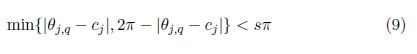
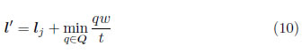
Where θj,q is the angle of the j-th candidate frequency bin for the q-th adjustment, that is, θj,q is related to the q-th candidate frequency adjustment qw/t. Additionally, the above calculation converges if β is chosen at random from the set 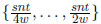 with small enough threshold s. Finally, the frequency location stage selects the minimum q from the set Q={q [t] | vj,q > Rloc/2 }; thus the estimated j-th permuted-frequency bin is refined using Eq. 10
2.2.4 Procedure EstimateValues This procedure, presented in Alg. 5, calculates the DFT estimation adjustment  , and it has the following input parameters: the time domain signal x; the instantaneous estimation of ; the parameter B; the flat window parameters δ and α; the set of located sparse components L; the number of sparse components to estimate K′; and the number of estimation iterations Rest.
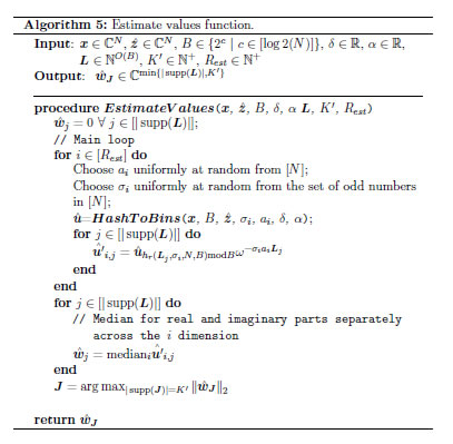
This procedure calculates the DFT estimation adjustment using three processing stages: the first one calculates the Rest sets of hashes-error from the signal x by using the procedure HashToBins and considering different pseudo-random permutation parameters; the second one separately calculates the median of the real and imaginary parts of the calculated hashes-error by only considering the set of located sparse frequency bins in L [1],[7], and by cancelling the pseudo-random spectral permutation; and the third one saves the K′ most energetic components .
3 Modified nearly optimal Sparse Fast Fourier Transform algorithm
In this section we describe the Modified Nearly Optimal sFFT algorithm and its optimized software implementation named sFFT-4.0, this implementation presents an improved accuracy compared with the original description [2].
3.1 Description of the modified nearly optimal sFFT algorithm
The modified sFFT algorithm is accomplished by designing a different flat window and by performing several modifications to the procedures described in section 2.
3.1.1 Modified flat window
In this case, we designed a flat window of the form (1/B,1/2B,δ, O(B log(N/δ))) as the one described in [1], and considering the time domain and DFT domain representations. The time domain representation of the flat window is described in Eq. 11, and this window does not depend on the parameter α and its support only depends on the parameters B and δ.
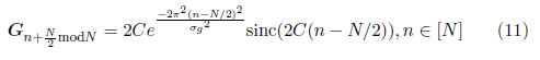
In this case, the flat window in time domain has a small support given by O(B log(N/δ)) and it is designed with an ideal low-pass filter using a Gaussian window with finite duration to truncate the impulse response. The cutoff frequency of the low-pass filter is 2C, where C is defined in Eq. 12 and the standard deviation of the Gaussian window is defined in Eq. 13.
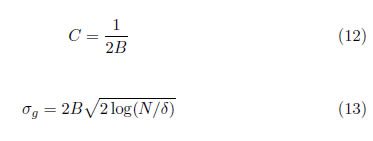
The DFT domain representation the flat window is described in Eq. 14.
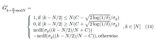
Where the vector is the approximated flat window and ncdf(x) = erfc is the Normal Cumulative Distribution Function [13]. In this case, satisfies
  < δ, and it has a flat super-pass region, a transition band of width 2
 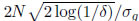 , and a total bandwidth of =
  which satisfies ≤ 2 N/B.
3.1.2 Modified procedure HashToBins
This modified procedure is shown in Alg. 6 by considering the designed flat window.
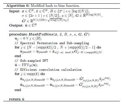
In this case, due to the designed flat window has a doubled bandwidth, each sparse component has two hashes located in the offsets of(j,σ,N,B) and oc(j,σ,N,B) given by the Eqs. 15 and 16, respectively.
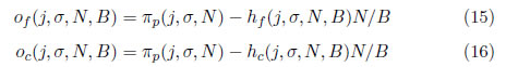
Where hf(j,σ,N,B)=  is the floor-hash function and hc(j,σ,N,B)=
  is the ceil-hash function; hf(j,σ,N,B) mod B and hc(j,σ,N,B) mod B are indexes of the two hashes in for a single sparse component of x. The proposed flat window improves the accuracy of the algorithm by solving the problem of the zero-value hashes, and it reduces the sampling cost by considering a smaller support.
3.1.3 Modified procedures LocateSignal and LocateInner
These modified procedures are presented in Alg. 7 and Alg. 8, respectively. In this case, we reduced the number of modified procedure HashToBins used by the modified procedure LocateInner by fixing the parameter a of the pseudo-random spectral permutation; this allows the usage of the same hashes-error for all the iterations of the modified procedure LocateInner, thus the sampling cost and the speed are improved.
3.1.4 Modified procedure EstimateValues This modified procedure, presented in Alg. 9, improves the estimation of the DFT values by adding a correction factor that cancels the effect of the windowing in DFT domain.
3.1.5 Modified procedure sFFT Taking into account the above improvements, the proposed modified Nearly Optimal sFFT algorithm is presented in Alg. 10, and it has the following input parameters: the time domain signal x, the sparsity order K, the parameter δ of the flat window [2], the location threshold s, and the number of estimation iterations (Rest).
The modified algorithm simplifies the calculation of the parameters B and K by halving their values during odd-numbered iterations (r mod 2 = 1), also the modified algorithm improves the accuracy of the DFT estimation .
4 Experimental results
We developed a software implementation of the modified sFFT algorithm named sFFT-4.0 [1],[2] by using the modified procedures HashToBins, LocateSignal, LocateInner, and EstimateValues. The Linux-based software implementation was developed using C language, the Intel® C Compiler, OpenMP [14], and the Intel MKL library; it was tested on one node of the Adroit cluster at Princeton University by using eight cores; and it was integrated with MATLAB® by using MEX-files shared libraries. We used OpenMP in some portions of the code in order to execute up to eight calls of the procedure HashToBins in parallel, hence we parallelized the main for-loops of the procedures LocateInner and EstimateValues. The source code of sFFT-4.0 is available at https://sourceforge.net/projects/sfft40/.
Finally, in order to test the performance of sFFT-4.0 implementation; first, we developed some comparisons of sFFT-4.0 implementation against the previous sFFT implementations AAFFT and sFFT-2.0 in terms of runtime and accuracy versus Signal to Noise Ratio (SNR); and second, we present the achieved improvements when the multicore architecture is used for sFFT-4.0 implementation.
4.1 Comparison tests
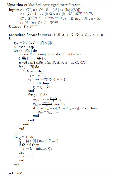
Figure 1(a) shows simulation results of the runtime versus N for K=50; where, red plot represents the runtime of sFFT-4.0 using a single core, the blue plot represents the runtime of sFFT-2.0 [1], and the green plot represents the runtime of AAFFT [7]. Even though our implementation is running on a single core, it is faster than AAFFT for all N values and faster than sFFT-2.0 for N ≥ 218.
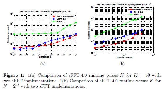
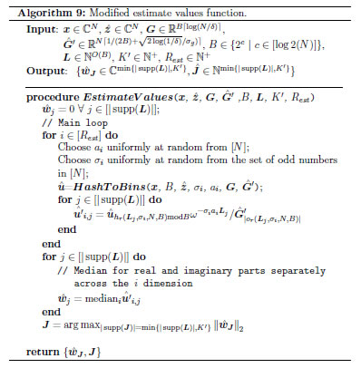
Figure 1(b) shows the simulation results of the runtime versus K for N=222; in this case, sFFT-4.0 is faster than AAFFT and sFFT-2.0 for all K values.
Figure 2 shows the simulation results of the l1-error versus SNR for N=222 and K=50; where the blue plot represents the error for sFFT-4.0 and the red plot represents the error for sFFT-2.0, the results for AAFFT are not worthy and were not included due to this algorithm is extremely sensitive to noise.
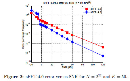
From 2 it can be seen that for values of SNR greater than −3 dB sFFT-4.0 has improved accuracy when compared with sFFT-2.0.
4.2 Multicore tests
Figure 3(a) shows simulation results of the runtime versus N for K=50; where, red plot represents the runtime of FFTW3 [8], the blue plot represents the runtime of sFFT-4.0 when one core is used, and the the green plot represents the runtime of sFFT-4.0 when eight cores are used. In this case, sFFT-4.0 is faster than FFTW3 for N above to 216 in the eight cores case; however, there is no a significant speed improvement by using the multicore architecture, this is due to the low sparsity of signal that leads to for-loops with small number of iterations which do not take advantage of the multicore architecture, hence the OpenMP's overhead times have a strong influence on the overall execution time [14].
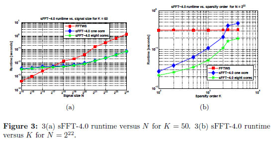
Figure 3(b) shows the simulation results of the runtime versus K for N=222; in this case, sFFT-4.0 is faster than FFTW3 for K below to 2500 when a single core is used. From Figure 3(b), it can be noted that there is a significant speed improvement by using the multicore architecture due the increased sparsity of signal; in this case we achieved an acceleration near to 4 ×.
Finally, the modified sFFT algorithm uses the following arithmetic operators: FFT, multiply-accumulate, trigonometric functions (sine, cosine, atan, atan2), modular inversion based on the Fermat's Little Theorem, among others; these operators can be easily mapped to hardware, thus this advantage could facilitate the implementation of the modified sFFT algorithm on an FPGA or an ASIC.
5 Conclusions
In this paper we present a modified Nearly Optimal sFFT algorithm for the noisy case, this algorithm reduces the sampling cost and corrects the zero-hash issue of the original algorithm by doubling the bandwidth of the flat window and by modifying the original procedures. Additionally, we developed an efficient software implementation of the modified Nearly Optimal sFFT algorithm using a multicore platform, under certain conditions this implementation is faster than the optimized FFT library FFTW3 and previous sFFT implementations. To the best knowledge of the authors, the developed implementation is the first one of the Nearly Optimal sFFT algorithm for the noisy case reported in literature. Finally, the future work will be addressed to perform an efficient hardware implementation of the modified Nearly Optimal sFFT algorithm using an FPGA.
Acknowledgement
Alexander López-Parrado thanks Colciencias for the scholarship and Universidad del Quindío for the study commission.
References
[1] H. Hassanieh, P. Indyk, D. Katabi, and E. Price, "Simple and practical algorithm for sparse Fourier transform," in ACM-SIAM Symposium on Discrete Algorithms (SODA). Kyoto, Japan: SIAM, 2012, pp. 1183-1194. [Online]. Available: http://dl.acm.org/citation.cfm?id=2095116.2095209 [ Links ]
[2] H. Hassanieh, P. Indyk, D. Katabi, and E. Price, "Nearly optimal sparse Fourier transform," in Proceedings of the 44th symposium on Theory of Computing (STOC), New York, USA, May 2012, pp. 563-578. [ Links ]
[3] P. Indyk, M. Kapralov and Eric Price, "(Nearly) Sample-Optimal Sparse Fourier Transform," in ACM-SIAM Symposium on Discrete Algorithms (SODA), Portland, USA, 2014. [ Links ]
[4] H. Hassanieh, L. Shi, O. Abari, E. Hamed, and D. Katabi, "GHz-wide sensing and decoding using the sparse Fourier transform," in INFOCOM, 2014 Proceedings IEEE. IEEE, 2014, pp. 2256-2264. [ Links ] [Online]. Available: http://dx.doi.org/10.1109/INFOCOM.2014.6848169
[5] A. C. Gilbert, S. Muthukrishnan, and M. J. Strauss, "Improved time bounds for near-optimal sparse Fourier representations," in Proceedings of SPIE Wavelets XI, San Diego, USA, 2005, pp. 1-15. [ Links ]
[6] A. C. Gilbert, Y. Li, E. Porat, and M. J. Strauss, "Approximate sparse recovery: optimizing time and measurements," in Proceedings of the 42nd ACM symposium on Theory of computing, Cambridge, USA, 2012. [ Links ]
[7] A. C. Gilbert, M. J. Strauss, and J. A. Tropp, "A Tutorial on Fast Fourier Sampling," IEEE Signal Processing Magazine, vol. 25, no. 2, pp. 57-66, 2008. [ Links ] [Online]. Available: http://dx.doi.org/10.1109/MSP.2007.915000
[8] M. Frigo and S. G. Johnson, FFTW, 3rd ed., Massachusetts Institute of Technology, 2012. [ Links ] [Online]. Available: http://www.fftw.org/
[9] C. Wang, M. Araya-Polo, S. Chandrasekaran, A. St-Cyr, B. Chapman, and D. Hohl, "Parallel Sparse FFT," in Proceedings of the 3rd Workshop on Irregular Applications: Architectures and Algorithms, New York, NY, USA, 2013, pp. 10:1--10:8. [ Links ] [Online]. Available: http://dx.doi.org/10.1145/2535753.2535764
[10] J. Hu, Z. Wang, Q. Qiu, W. Xiao, and D. J. Lilja, "Sparse Fast Fourier Transform on GPUs and Multi-core CPUs," in Computer Architecture and High Performance Computing (SBAC-PAD), 2012 IEEE 24th International Symposium on, Oct. 2012, pp. 83-91. [ Links ] [Online]. Available: http://dx.doi.org/10.1109/SBAC-PAD.2012.34
[11] J. Schumacher, "High Performance Sparse Fast Fourier Transform," Master Thesis, ETH Zurich, Department of Computer Science, 2013. [ Links ] [Online]. Available: http://goo.gl/3alHvS
[12] A. Dutt and V. Rokhlin, "Fast Fourier transforms for nonequispaced data, II," Applied and Computational Harmonic Analysis, vol. 2, no. 1, pp. 85-100, 1995. [Online]. Available: http://dx.doi.org/10.1006/acha.1995.1007 [ Links ]
[13] M. Abramowitz and I. A. Stegun, Handbook of Mathematical Functions with Formulas, Graphs, and Mathematical Tables, 10th ed. Washington, DC, USA: Dover, 1972. [ Links ]
[14] OpenMP, OpenMP Application Program Interface, OpenMP Architecture Review Board Std., 2013. [ Links ]
