ARTÍCULO DE REVISIÓN

DOI: 10.17230/ingciencia.11.22.10

Prediction of Multiphase Flow in Pipelines: Literature Review

Predicción del flujo multifásico en tuberías: artículo de revisión

M. Jerez-Carrizales¹, J. E. Jaramillo² and D. Fuentes³

1 Universidad Industrial de Santander, Bucaramanga, Colombia, manuel.jerez@correo.uis.edu.co.

2 Universidad Industrial de Santander, Bucaramanga,Colombia, jejarami@uis.edu.co.

3 Universidad Industrial de Santander, Bucaramanga, Colombia, dfuentes@uis.edu.co.

Received: 06-05-2015 Accepted: 02-07-2015 Online: 31-07-2015

MSC:76T10 PACS:47.55.Ca

Abstract

In this work a review about the most relevant methods found in the literature to model the multiphase flow in pipelines is presented. It includes the traditional simplified and mechanistic models, moreover, principles of the drift flux model and the two fluid model are explained. Even though, it is possible to find several models in the literature, no one is able to reproduce all flow conditions presented in the oil industry. Therefore, some issues reported by different authors related to model validation are here also discussed.

Key words: drift flux; two fluid; mechanistic; vertical lift performance; pressure drop

Resumen

En este trabajo se presenta una revisión de los métodos más relevantes en la industria del petróleo para modelar el flujo multifásico en tuberías. Se incluyen desde los modelos simplificados hasta los modelos mecanicistas además de explicar los principios de los modelos drift flux y two fluid. Existe una gran cantidad de modelos en la literatura para simular el flujo multifásico en tuberías, empero, ningún modelo es capaz de reproducir todas las condiciones de flujo multifásico presentes en la industria del petróleo. Finalmente, se mencionan algunos temas en los que se requiere más investigación que lleven a simulaciones con resultados más cercanos a los datos de pozos reales.

Palabras clave: tubería; modelo drift flux; dos fluidos; mecanicistas; caída de presión

1  Introduction

Generally, models applied to predict tubing performance relationship (TPR) can be classified as large-scale models and small scale models. The large scale models are based on space averaging. They are developed to obtain a representative value of the velocity and the pressure in a given region. The most common large scale models are homogeneous, drift-flux and two-fluid models. On the other hand, the small scale models simulate the multiphase flow tracking the interface, they can show bubbles, slugs and their shapes. This means that they are more computational time demanding. Some ideas were explained behind new techniques such as Hybrid Direct Numerical Simulation (HDNS) and Lattice Boltzmann method [1] .

The large scale models are chronologically classified[2] as :

1. The Empirical Period, 1950-1975: in this period some empirical correlations were developed, in which, mixture was treated as a homogeneous one. These correlations were based on a few experiments made on laboratories and fields. Moreover, some researchers noticed flow patterns in two-phase flows and slippage between phases. Some correlations were published in this period of time by [3],[4],[5],[6] and [7]. In spite of the time, modified Hadegorn & Brown methods were still recommended to calculate the pressure drop in vertical pipes in the 90's [8][9].

2. The Awakening Years, 1970-1985: personal computers were used in these years by companies to predict flow rates and pressure distribution in pipelines. Besides, flow pattern selection were not successful, and the flow in inclined pipes was not well predicted. Some works were presented in this period of time by [10],[11] and [12].

3. The Modeling Period, 1980 - 1994: physics involved in multiphase flow was better understood and some mechanistic models were developed. Furthermore, new experiments were carried out with improved instruments. Some examples of works in this period are [13],[14] and [8]. Governing equations were also defined for each phase: mass conservation, momentum conservation and energy conservation. In addition, new transient methods started to find their way. Finally, new commercial software was created to solve these equations.

   The final date of the Modeling Period was set in [2] because publication year of article, however, investigations in the last two decades are focus on similar topics: reliable data from new flow loops, elaborated models to represent physics, corrections in the flow pattern maps and simplified models with tunning capabilities. Different kind of models has been implemented, it includes simple models as well as more elaborated models. Some mechanistic models for deviated wells were presented by [15],[16],[17] and [18]. An example of a drift flux model developed in this period of time was done by [19].

2  Mechanistic and simplified models

There are two main groups where most of models can be classified, they are mechanistics models and simplified models. No matter which kind is, all models get as their results the value of pressure drop per unit length and they generally include the calculation of the holdup and flow pattern. Furthermore, most of them use an hydrodynamic approach not a thermodynamic one.

In simplified models, a set of empirical correlations is developed to obtain the mentioned results. Some of these equations do not have a physical ground, they are adjusted using experimental data. In comparison, mechanistic models propose a momentum balance equation for each flow pattern presented, then, a group of equations must be solved. Nevertheless, the mechanistic models still need some empirical relations. In the following sections the drift flux model and the two fluid model are explained. The drift flux model is an special case of the simplified model and the two fluid model is also an important mechanistic model.

Another classification of the models are steady and unsteady state models. Steady state models do not need a mass balance equation, also, properties are averaged in a piece of the pipe, and the superficial velocities are calculated from a volumetric flux at standard conditions. On the other hand, unsteady state models have to calculate the outflow in the pipe.

The first attempts to predict the vertical wellbore performance were published in [3] and [20]. They used an empirical equation to determine the pressure gradient. This equation depends on hydrostatic pressure and friction factor, each author presented a graph to calculate the last one. Main constraint of these models is assumption of an homogeneous mixture, which is not valid for all flow patterns, i.e., slug flow pattern in which an slippage exists between phases.

A group of dimensionless numbers was defined by [4]. They also developed a model based on them. Equally important, they described a flow pattern map with three main regions.

Two years later, a 1500 [ft] deep vertical well in Dallas was used to make a test with air, water and oil as working fluids [7]. They also used data from [5] to sum 475 tests or 2905 pressure points. This method is used for vertical flow and it has been selected several times by different authors as starting point for new models. For example, the modified Hagedorn & Brown method¹ exhibited an excellent performance against another models and data [8]. One of those modifications counteracts a physically impossible value for the liquid holdup² for upward flow; the original Hagedorn & Brown method can incorrectly predict a higher velocity for the liquid phase than the gas phase. The modified method set both velocities to the same value instead [21].

An extension of a model developed in [22] was proposed by [6]. Orkiszewski used the Griffith & Wallis model for bubble flow pattern and the Duns & Ros model for mist flow. Furthermore, he used data collected in [7]. Afterwards, the model [6] was modified by [11] in the slug-froth regime. The first correlation which can be used for deviated wells was developed by [12]. They used an acrylic pipe of 90 [ft] long with 1 [in] and 1.5 [in] diameter, and they carried out 584 tests for different angles using air and water.

The first mechanistic model was developed by [23], since then, several methods have been published, i.e., [8] and [15]. In 1994, a mechanistic model based on several methods was developed to describe mathematically flow patterns [8]. The flow pattern prediction was based on works of [24] and [25]. Finally, the model was compared with 1712 well cases from several origins and 7 methods. Ansari et al. found a better performance than the others 7 models, however, performance of 4 methods were comparable to. It should be noted that Ansari method was not focused on deviated wells, it could result in a greater percentage of error.

Another mechanistic model was defined by [15], this model took into account the following flow patterns: dispersed bubble flow, stratified flow, annular mist flow, bubble flow, slug flow, and froth flow. Froth flow is calculated as an interpolation of dispersed bubble flow and annular mist or slug flow and annular mist, this solves discontinuity problems caused by transitions between flow patterns. They used a data base with 20000 laboratory measurements and 1800 measurements from wells.

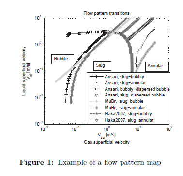
An example of three methods to select flow pattern is shown in the Figure 1. The flow pattern map is generated using a home made code developed by the authors applying [8],[24],[25],[13],[19]. It is a qualitative example that shows the existence of some discrepancies between these methods.

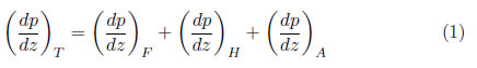
A general equation that shows sources of the pressure drop in steady state is written in (1). The total pressure drop depends on friction lost, height and acceleration of the fluid. Accelerating pressure gradient (last term in 1) can be caused by the expansion of the fluid or by inflow/outflow through the wall pipes [26],[9].

Most of the old models were focused on vertical flow (vertical-lift performance) or horizontal flow. A comparison of 16 correlations³ for horizontal flow was made against 10500 pressure drop data [27]. A comparison of 8 correlations for vertical and deviated pipes was made by [8]. Results on deviated wells were not satisfactory.

The works found in the literature use data from laboratories and real fields to develop the models presented. 23 laboratory flow loops were compared to study multiphase flow based on a broad range of data [28]. They used 6 criteria: total reported length, maximum working diameter, inclination, operating pressure, length of vertical test section and type of fluid. They searched information available in the scientific literature about these 23 flow loops. Eventually, they suggested some necessary factors that must be considered to standardize the capabilities of flow loops. This information allows to assess different models in a wide range of situations.

A review of several models to predict the pressure drop and heat transfer in pipelines is presented in [29]. Most of the models presented were related to the refrigeration industry and they conclude that the average error of models's prediction is 25%.

3  Drift-flux model

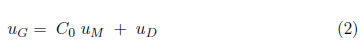
One of the large scale models is the drift flux approach. In some cases of multiphase flow, slippage between phases can be determined accurately with a basic equation called drift flux model (2). The equation (2) describes a relation between the gas velocity and the mixture velocity using the drift velocity u_D and the distribution parameter C₀ [30].

The most common cases occur when relative velocity is caused by buoyancy or drag force. Studies about applicability of (2) for liquid-gas flow under certain conditions was made by [31],[32], [33],[34] among others, as it was recently explained in [35].

Another study which investigated utilization of (2) was done by [36], as result of their work, they obtain other values to the distribution parameter and drift velocity as a function of void fraction, velocities, densities and inclination angle. They used data from a flow loop with a pexiglass pipe, a diameter of 15.2 [cm] and a length of 11 [m] at different angles, this diameter is commonly used in oil industry but it is not common for testing purposes. The drift flux parameters were optimized with a balance between complexity and closeness of fit. Their model is only valid for water/gas and oil/water for a pipe diameter of 15.2 [cm]. However, it is necessary to modified their model if it is used for different conditions, but, they do not present the needed modifications. Finally, important discrepancies with some data of oil/water experiment were found corresponding to oil fraction around 75%.

An iterative procedure is explained in [37] about three phase (oil-water-gas) flow. They find first the void fraction with a representative liquid mixture and then, they calculate the holdup of every liquid. They found that oil-water mixture can be assume as an homogeneous liquid phase (without slippage) in a oil-water-gas flow when pipe is vertical or near vertical and volume gas fraction is greater than 0.1.

The drift flux approach (2) solves a kinematic problem. For that reason, conservative equations are applied to the mixture as a homogeneous model [38] with a slippage. Therefore, a complex problem (two phase flow with coupled equations) is solved in an easy way using the drift flux model.

An homogeneous model, a drift flux model and a segmented approach was used by [26] to calculate the pressure drop in a wellbore. The pressure gradient is calculated as a combination of friction, gravity, wall inflow⁴ and expansion pressure drop. The drift-flux equation applied was proposed by Mishima and Ishii (1984), this equation is flow pattern independent.

Another example of the drift flux approach is proposed by [19]. This drift flux model is flow pattern dependent and it was assumed no slippage in annular flow.

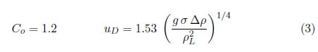
Each author defines a value or a function for the distribution parameter and the drift velocity. These values were defined by [32] as (3).

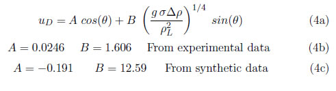
Another values of C_o and u_D were presented by [39], (see equation 4). They also showed 9 drift flux models. They used 1000 data from seven TUFFP (Tulsa University Fluid Flow Project) two-phase experiments: 5 experiments were used to develop their model (4b) and 356 data from two experiments were used to test their model. Moreover, they used 463 data from OLGA (OiL and GAs simulator) Multiphase Toolkit to find another values to the drift velocity (4c). They used the same value for C_o in both works. Furthermore, equation (4a) is valid for different inclination angles of the pipe. The difference between coefficients A and B for both experimental data and synthetic data are shown in (4b) and (4c). Therefore, in a vertical pipe, drift velocity calculated from constants of synthetic data is 7 times larger than that evaluated using constants from experimental data.

Values from experimental data were used in [35] to develop a fast transient solver with a power law method in order to find the pressure drop. The power law method, which is a modified version of that proposed in [40], is a simple formula that can be applied to a wide range of multiphase flows. Moreover, the Choi et al. model involves more constants that can be easily tuned, what can lead to a better performance for specific cases. Other example of a drift flux model with tunning capabilities is presented in [41]. They used the ensemble Kalman filter technique to set some constants from experimental data in real time for underbalanced and low head drilling. However, experimental data were not available at the pipeline design time [42]. Thereby, calibration is not possible at the design time. According to [38], these models can be applied as long as temporal variations are small enough.

The model of [35] is based on a quasi steady state. Therefore, this approach can not predict fast changes in the flow pattern, and some discrepancies with experimental data are observed in the early stages of the simulation, when temporal changes are more notorious. Its simplicity imply that solution can be found fast. Another transient drift flux simulators are present by [43],[44],[45]. In these works a thermal analysis is also carried out. Mao & Harvey and Livescu calculate the mass and energy balance equation in transient state and the pressure gradient in steady state; Han et al. use a transient gradient pressure equation and the overall method of solution was Newton iterations, this solution method was used by Livescu. On the other hand, Mao & Harvey use a three phase flash calculation to get properties of the crude instead of the black oil model, which was used by Han et al..

4  Two Fluid Model (TFM)

In a two fluid model, a set of conservative equations is used for each fluid (phase). In this work, formulation and notation used in [38] have been selected, and it is used in what follows.

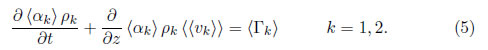
The continuity equation (5) is formed by a transient term (temporal derivative), a convective term (spatial derivative) and a change of phase term. The Γ_k cause the couple of the two continuity equations because the lost mass of the k-fluid per unit volume and unit time is equal to the gain of the mass of the other fluid. The change of phase term is used by [46],[47],[48],[49] and it is assumed negligible by [50],[51],[52],[53],[54].

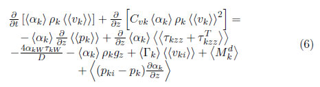
The momentum conservation equation (6) [38] in the right hand side contains: the pressure gradient in the flux direction, the gradient of the mean shear stress in the flux direction, the shear stress with the wall of the pipe, the gravitational force, the force due to the change of phase, the total interfacial shear force, the force due to difference in the pressure from the interface concerning to the mean value (important for horizontal stratified flow [38]). The total interfacial shear force is the linkage into the two momentum conservation equations. The first term depending of the shear stress is not used in most of the 1-D analysis [51],[46],[52],[50],[48],[54].

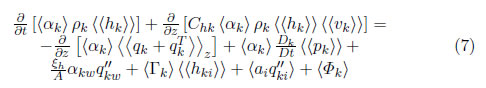
Finally, the energy conservative equation (in terms of enthalpy) is presented in (7) [38]. Terms of the right hand side of the equation are: heat flux by conduction in the fluid, pressure energy, heat flux by the wall, enthalpy of the change of phase mass, heat flux in the interface of the two fluids and the viscous dissipation. Neither Morales-Ruiz et al. nor Cazarez-Candia et al. include the viscous dissipation term, however, Cazarez-Candia et al. include the potential energy in their equations which is not listed in (7).

Not all models include in their analysis the energy conservative equations. Some authors assume isothermal analysis [51],[46],[52] or adiabatic conditions [50] from the wall of the pipe, other authors used only one mixture energy conservative equation in spite of develop an hydraulic two fluid model [54]. A comparison of different thermal assumption in the thermal model was made by [55]. In (7), the heat flux in the wall q_kw can be assumed to be equal to the heat flux in the ground, but it is recommended taking into account the energy storage of the tubing and the casing [56].

Different algorithms are applied to solve the system of equations for the given set of boundary and initial conditions. Two of the most used methods are Newton iteration [54] and pressure correction scheme [46],[57]. The pressure correction schemes can cause convergence problems due to linkage between equations, some modifications for the SIMPLE method are explained by [48] to avoid some convergence problems.

In addition to the equation system, the solution of a two fluid model is harder to found than the one of the drift flux model because there are more coupled equations. Likewise, the two fluid model can get better results for simulation with changing conditions than the drift flux model. Therefore, the two fluid model is recommended for transient phenomena, wave propagations and flow regime changes [38].

A numerical analysis of the two fluid model near ill posedness was made by [57]. In horizontal flow, flow pattern can change from stratified flow to slug flow when slip velocity is greater than a critical value, this instability is known as Kelvin-Helmholtz (KH). An additional issue to the KH instability is presented when balance equations are solved numerically. It is evaluated instability of 1st-order upwind, 2nd-order upwind, central difference scheme and QUICK scheme with a Von Neumann stability analysis. Counterintuitively, it was found that the central difference scheme is more accurate and stable than the others, so, high order schemes are not always the best option from a convergence point of view.

In a one dimensional TFM discretized with a finite difference method (FDM), it is defined pressure and temperature from both fluids in the same node and these values can be different. Normally, this difference is negligible what was the assumption used by [54]. In contrast, an application of a different pressure on a control volume is shown by [52]. They presented a one-dimensional two fluid compressible model with a pressure relaxation arguing less instability problems. Also, in their work was used an Avdection Upstream Splitting Method (AUSMDV) with a Flux Difference Splitting (FDS) and a Flux Vector Splitting (FVS). The AUSMDV is said to be robust, accurate and stable near a change of one to two phase. The pressure difference is found with an additional equation for the evolution of the volume fraction.

The classical two fluid model defines a set of closure relations for each flow pattern and needs a previous flow pattern selection. It does not only add errors for a wrong selection of the flow pattern, but also discontinuities when flow regime change is simulated could appear. A new dynamic approach uses an interfacial area transport equation (IATE) [38].

Different flow pattern maps for different angle inclination was used by [54]: the flow pattern map of Ouyang(1998) for horizontal flow and the flow pattern map of Shoham (2006) for vertical flow. The flow pattern map for deviated wells is similar to the vertical one. They highlight importance of a correct selection of the flow pattern with an example, in which, stratified and bubbly flow was used to compare results against experimental data.

Some works are focused on a specific flow pattern [50]. They developed a model for slug flow in two steps, the first one is the liquid slug which is modeled like a bubbly flow, while the second part (Taylor bubble) is modeled like a stratified flow (pipe angle lesser than 45° from horizontal) or annular flow (angle bigger than 45°).

The interfacial area transport (IAT) approach does not use a traditional flow pattern selection. It works with two groups, the first group represents spherical and distorted bubbles while the second group represents cap, slug and churn bubbles [38]. It means that two gas momentum equations should be solved, specially, in three dimensional analysis. In contrast, in one dimensional analysis, the two gas momentum equations can be mix to get only one gas momentum equation. This equation needs an additional closure relation to determine the velocity difference for the groups, a drift flux model can be used for that purpose [58]. A one group interfacial area transport equation in the TRACE code was implemented by [59] for the nuclear industry. They found an improvement on the bubble prediction compared with the traditional TRACE, but, the pressure gradient and the void fraction were found to be nearly the same. A formulation of the drift flux approach and the drag coefficient approach was presented to calculate the interfacial momentum transfer in the momentum conservation equation for an IAT approach in [60].

5  Challenges and issues

10 challenges was proposed by [61]. Most of them have been investigated, however, there are still some topics that must be addressed. Fluid properties and flow pattern prediction specially at high pressure and high temperature (HPHT) are two of them.

Regarding fluid properties, some lines of research of the National Energy Technology Laboratories (NETL) was explained by [62] and the need of a fluid database (oil with other components such as hydrogen sulfide, among others) at high pressure and high temperature. This database will help to evaluate existing correlations and creates new ones.

Regarding flow pattern, an example of a wrong selection of flow pattern at high pressure was given by [19], in which, annular flow is predicted when churn, slug and dispersed bubble flows are also possible. Also, some differences in the predicted flow pattern for high viscous flow was shown by [63],[64] and [65]. It was suggested by [1] that 3D simulation can be used to get a better understanding of flow pattern transitions.

The multiphase flow in pipelines is not an isolated problem, but it is one part of the production system in the oil industry. Two areas highlighted by [28] to be investigated are: sand transport in oil - gas and dynamic interactions between flow in porous media and flow in pipes under transient flow conditions. Modeling of three-phase gas-oil-sand flow is not well understood yet [66]. Moreover, facilities at large scale and high concentration of sand should be developed. It will help to prevent deposition of sand in pipes and other stuffs. On the other hand, a coupled facility for a pipeline and a reservoir under transient conditions should be developed, most of the models used are transient pipeline models with stable reservoir, this can yield to a wrong estimation of the reservoir pressure.

In addition, some cases in which terrain slugging was unsatisfactorily predicted by Commercial software were presented by [67].

There is not a method to predict properly wellbore performance in all cases. Advantages and disadvantages of every method should be taken into account, it will make that application of a method produce accurate or unsatisfactory results in some conditions.

6  Conclusions

The revision of the different methods shows a wide range of methods from simple to complex ones, with different accuracy for the simulation of the multiphase flow in pipelines.

The most complex methods for simulation of two phase flow not always imply the most accurate methods. Due to the variety of condition in the oil industry, it is necessary to assess models at conditions how they will be used.

Some methodologies are flow pattern dependent, it also implies that a wrong flow pattern selection means an additional error to the fluids velocities and the pressure gradient in the pipe. Some other methods are flow pattern independent, most of them present a mathematical advantage of being continuous.

The need of database and flow in special cases are topics that should be consistently investigated.

Acknowledgements

This work received financial support provided by VIE-CEC Vicerrectoría de Investigación y Extensión - Campo Escuela Colorado No. 8557, Universidad Industrial de Santander, and, Jóvenes Investigadores Colciencias No. 617. Also, it is expressed acknowledgments to the Escuela de Ingeniería Mecánica and the Grupo de Investigación en Energía y Medio Ambiente.

Footnotes:

¹The modified Hagedorn & Brown method used by Ansari is able to calculate pressure drop in deviated wells.

²The holdup is a ratio between transversal area occupied by liquid and total transversal area.

³10 correlations for all flow patterns and 6 correlations for specific flow patterns. 2 correlations of the 16 were based in data from the selected data base.

⁴ This model took into account flow in the walls

References

[17] A. Kaya, C. Sarica and J. Brill, "Mechanistic Modeling of Two-Phase Flow in Deviated Wells," SPE Production & Facilities, vol. 16, pp. 156-165, 2001.         [ Links ] [Online]. Available: http://dx.doi.org/10.2118/72998-PA 215

[36] H. Shi, J. Holmes, L. Diaz, L. Durlofsky, and K. Aziz, "Drift-Flux Modeling of Two-Phase Flow in Wellbores," SPE Journal, vol. 10, pp. 24-33, 2005.         [ Links ] [Online]. Available: http://dx.doi.org/10.2118/84228-PA 219

[60] C. Brooks, T. Hibiki, and M. Ishii, "Interfacial drag force in one-dimensional two-fluid model," Progress in Nuclear Energy, vol. 61, pp. 57-68, 2012.         [ Links ] [Online]. Available: http://dx.doi.org/10.1016/j.pnucene.2012.07.001 225

References

[1] O. F. Ayala, L. F. Ayala, and O. M. Ayala, "Multi-phase Flow Analysis in Oil and Gas Engineering Systems and its Modelling," Hydrocarbon World, pp. 57-61, 2007. [ Links ] 214, 225
[2] J. Brill and H. Mukherjee, Multiphase flow in wells. Texas: Henry L. Doherty Memorial Fund of AIME, Society of Petroleum Engineers., 1999. [ Links ] 214, 215
[3] F. Poettmann and P. Carpenter, "The Multiphase Flow of Gas, Oil, and Water Through Vertical Flow Strings with Application to the Design of Gaslift Installations," in Drilling and Production Practice. American Petroleum Institute, 1952, pp. 257-317. [ Links ] 214, 216
[4] H. J. Duns and N. Ros, "Vertical flow of gas and liquid mixtures in wells," in 6th World Petroleum Congress. World Petroleum Congress, 1963, pp. 451-465. [ Links ] 214, 216
[5] G. H. Fancher and E. Brown Kermit, "Prediction of Pressure Gradients for Multiphase Flow in Tubing," SPE Journal, vol. 3, no. 1, pp. 59-69, 1963. [ Links ] 214, 216
[6] J. Orkiszewski, "Predicting Two-Phase Pressure Drops in Vertical Pipe," Journal of Petroleum Technology, vol. 19, no. 6, pp. 829-838., 1967. [ Links ] 214, 217
[7] A. Hagedorn and K. Brown, "Experimental Study of Pressure Gradients Occurring During Continuous Two-Phase Flow in Small-Diameter Vertical Conduits," Journal of Petroleum Technology, vol. 17, no. 4, pp. 475-484, 1965. [ Links ] [Online]. Available: http://dx.doi.org/10.2118/940-PA 215, 216, 217
[8] A. M. Ansari, N. D. Sylvester, C. Sarica, O. Shoham and J. P. Brill, "A Comprehensive Mechanistic Model for Upward Two-Phase Flow in Wellbores," SPE Production & Facilities, vol. 9, no. 2, pp. 143-151, 1994. [ Links ] 215, 216, 217, 218
[9] A. R. Hasan and C. S. Kabir, Fluid Flow and Heat Transfer in Wellbores. Society of Petroleum Engineers, 2002. [ Links ] 215, 218
[10] K. Aziz, G. Govier and M. Fogarasi, "Pressure Drop in Wells Producing Oil and Gas," Journal of Canadian Petroleum Technology, vol. 11, no. 3, 1972. [ Links ] 215
[11] G. L. Chierici, G. M. Ciucci and G. Sclocchi, "Two-Phase Vertical Flow in Oil Wells - Prediction of Pressure Drop," Journal of Petroleum Technology, vol. 26, no. 8, pp. 927-938, 1974. [ Links ] 215, 217
[12] D. Beggs and J. Brill, "A Study of Two-Phase Flow in Inclined Pipes," Jour- nal of Petroleum Technology, vol. 25, no. 5, pp. 607-617, 1973. [ Links ] 215, 217
[13] H. Mukherjee and J. Brill, "Pressure drop correlations for inclined two-phase flow," Journal of energy resources technology, vol. 107, no. 4, pp. 549-554, 1985. [ Links ] 215, 217
[14] A. R. Hasan and C. S. Kabir, "Predicting Multiphase Flow Behavior in a Deviated Well," SPE Production Engineering, vol. 3, no. 4, pp. 474-482, 1988. [ Links ] [Online]. Available: http://dx.doi.org/10.2118/15449-PA 215
[15] N. Petalas and K. Aziz, "A Mechanistic Model for Multiphase Flow in Pipes," Society of Petroleum Engineers [successor to Petroleum Society of Canada], vol. 39, no. 6, 2000. [ Links ] 215, 217
[16] L. Gomez, O. Shoham, Z. Schmidt, R. Chokshi and T. Northug, "Unified Mechanistic Model for Steady-State Two-Phase Flow: Horizontal to Vertical Upward Flow," SPE Journal, vol. 5, pp. 339-350, 2000. [ Links ] 215