English (pdf)
 Article in xml format
 Article references
 Send this article by e-mail
 Cited by SciELO
  Cited by Google
  Similars in
SciELO
Similars in
SciELO  Similars in Google
 Permalink
1 Introduction
The gamma function was first introduced by Leonard Euler in 1729, as the limit of a discrete expression and later as an absolutely convergent improper integral, namely,
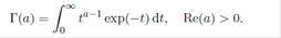 ()1
()1
The gamma function has many beautiful properties and has been used in almost all the branches of science and engineering.
One year later, Euler introduced the beta function defined for a pair of complex numbers a and b with positive real parts, through the integral
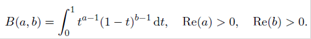 ()2
()2
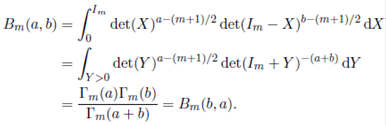
The beta function has many properties, including symmetry, B(a,b) = B(b,a), and its relationship to the gamma function,
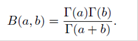
In statistical distribution theory, gamma and beta functions have been used extensively. Using integrands of gamma and beta functions, the gamma and beta density functions are usually defined.
Recently, the domains of gamma and beta functions have been ex- tended to the whole complex plane by introducing in the integrands of (1) and (2), the factors exp (−σ/t) and exp (−σ/t(1 − t)), respectively, where Re(σ) > 0. The functions so defined have been named extended gamma and extended beta functions.
In 1994, Chaudhry and Zubair (7 defined the extended gamma function,
Γ(a; σ), as
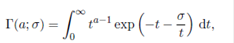 ()3
()3
where Re(σ) > 0 and a is any complex number. For Re(a) > 0 and σ = 0, it is clear that the above extension of the gamma function reduces to the classical gamma function, Γ(a, 0) = Γ(a). The extended gamma function is a special case of Krätzel function defined in 1975 by Krätzel 16. The generalized gamma function (extended) has been proved very useful in various problems in engineering and physics, see for example, Chaudhry and Zubair 8.
In 1997, Chaudhry et al. 6 defined the extended beta function
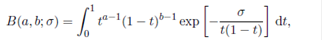 ()4
()4
where Re(σ) > 0 and parameters a and b are arbitrary complex numbers. When σ = 0, it is clear that for Re(a) > 0 and Re(b) > 0, the extended beta function reduces to the classical beta function B(a, b).
Recently, Özergin, Özarslan and Altın 24 have further generalized the extended gamma and extended beta functions as
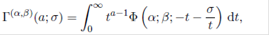 ()5
()5
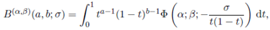 ()6
()6
where Φ (α; β; ·) is the type 1 confluent hypergeometric function. The gamma function, the extended gamma function, the beta function, the extended beta function, the gamma distribution, the beta distribution and the extended beta distribution have been generalized to the matrix case in vaious ways. These generalizations and some of their properties can be found in Olkin 23, Gupta and Nagar 10, Muirhead 18, Nagar, Gupta, and Sánchez 19, Nagar, Roldán-Correa and Gupta 20, Nagar and Roldán- Correa (21), and Nagar, Morán-Vásquez and Gupta 22. For some recent advances the reader is refereed to Hassairi and Regaig 12, Farah and Hassairi 4, Gupta and Nagar 11, and Zine 25. However, generalizations of the extended gamma and extended beta functions defined by (5) and (6), respectively, to the matrix case have not been defined and studied. It is, therefore, of great interest to define generalizations of the extended gamma and beta functions to the matrix case, study their properties, obtain different integral representations, and establish the connection of these generalizations with other known special functions of matrix argument.
This paper is divided into seven sections. Section 2 deals with some well known definitions and results on matrix algebra, zonal polynomials and special functions of matrix argument. In Section 3, the extended matrix variate gamma function has been defined and its properties have been studied. Definition and different integral representations of the extended matrix variate beta function are given in Section 4. Some integrals involving zonal polynomials and generalized extended matrix variate beta function are evaluated in Section 5. In Section 6, the distribution of the sum of dependent generalized inverted Wishart matrices has been derived in terms of generalized extended matrix variate beta function. We introduce the generalized extended matrix variate beta distribution in Section 7.
2 Some known definitions and results
In this section we give several known definitions and results. We first state the following notations and results that will be utilized in this and subsequent sections. Let A = (aij ) be an m × m matrix of real or complex numbers. Then, At denotes the transpose of A; tr(A) = a 11 +· · · + amm ; etr(A) = exp(tr(A)); det(A) = determinant of A; "A" = spectral norm of A; A = At > 0 means that A is symmetric positive definite, 0 < A < Im means that both A and Im − A are symmetric positive definite, and A 1 / 2 denotes the unique positive definite square root of A > 0.
Several generalizations of the Euler's gamma function are available in the scientific literature. The multivariate gamma function, which is frequently used in multivariate statistical analysis, is defined by
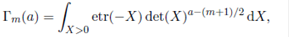 ()7
()7
where the integration is carried out over m× m symmetric positive definite matrices. By evaluating the above integral it is easy to see that
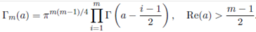 ()8
()8
The multivariate generalization of the beta function is given by
 ()9
()9
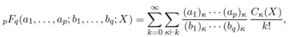
The generalized hypergeometric function of one matrix argument as defined by Constantine 9 and James 15 is
 ()10
()10
where Cκ(X) is the zonal polynomial of m×m complex symmetric matrix X corresponding to the ordered partition κ = (k 1 , . . . , km ), k 1 ≥ · · · ≥ km ≥ 0, k 1 + · · · + km = k and denotes summation over all partitions κ. The generalized hypergeometric coefficient (a) κ used above is defined by
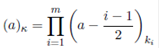 ()11
()11
where (a)r = a(a + 1) · · · (a + r − 1), r = 1, 2, . . . with (a)0 = 1. The parameters ai, i = 1, . . . , p, bj , j = 1, . . . , q are arbitrary complex numbers.
No denominator parameter bj is allowed to be zero or an integer or half- integer ≤ (m−1)/2. If any numerator parameter ai is a negative integer,
a 1 = −r, then the function is a polynomial of degree mr. The series converges for all X if p ≤ q, it converges for ||X|| < 1 if p = q + 1, and, unless it terminates, it diverges for all X ƒ= 0 if p > q.
If X is an m × m symmetric matrix, and R is an m × m symmetric positive definite matrix, then the eigenvalues of RX are same as those of R 1 / 2 XR 1 / 2, where R 1 / 2 is the unique symmetric positive definite square root of R. In this case Cκ (RX) = Cκ (R 1 / 2 XR 1 / 2) and
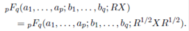 ()12
()12
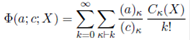
Two special cases of (10) are the confluent hypergeometric function and the Gauss hypergeometric function denoted by Φ and F , respectively. They are given by
and
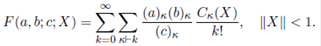 ()13
()13
The integral representations of the confluent hypergeometric function Φ and the Gauss hypergeometric function F are given by
 ()14
()14
and for X < Im,
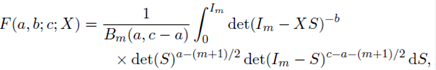 ()15
()15
where Re(a) > (m − 1)/2 and Re(c − a) > (m − 1)/2.
For properties and further results on these functions the reader is referred to Herz 13, Constantine 9, James 15, and Gupta and Nagar 10.
The confluent hypergeometric function Φ satisfies the Kummer's relation
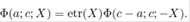 ()16
()16
From (15), it is easy to see that
Lemma 2.1. Let Z be an m×m complex symmetric matrix with Re(Z) > 0 and let Y be an m × m complex symmetric matrix. Then, for Re(t) > (m − 1)/2, we have
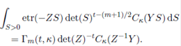 ()17
()17
Lemma 2.2. Let Z be an m×m complex symmetric matrix with Re(Z) > 0 and let Y be an m × m complex symmetric matrix. Then, for Re(t) > k 1 + (m − 1)/2, we have
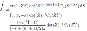 ()18
()18
Lemma 2.3. Let Y be an m × m complex symmetric matrix, then for Re(a) > (m − 1)/2 and Re(b) > (m − 1)/2, we have
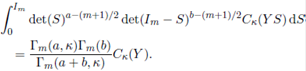 ()19
()19
Lemma 2.4. Let Y be an m × m complex symmetric matrix. Then
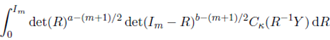
 ()20
()20
where Re(a) > k 1 + (m − 1)/2 and Re(b) > (m − 1)/2.
Results given in Lemma 2.1 and Lemma 2.3 were given by Constantine 9 while Lemma 2.2 and Lemma 2.4 were derived in Khatri 17. In the expressions (17) and (18), Γ m (a, ρ) and Γ m (a, −ρ), for an ordered partition ρ of r, ρ = (r1, . . . , rm), are defined by

and
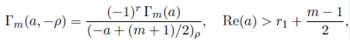
respectively.
Definition 2.1. The extended matrix variate gamma function, denoted by Γm(a; Σ), is defined by
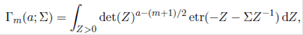 ()21
()21
where Re(Σ) > 0 and a is an arbitrary complex number.
From (21), one can easily see that for Re(Σ) > 0 and H ∈ O(m), Γ m (a; HΣH') = Γ m (a; Σ) thereby Γ m (a; Σ) depends on the matrix Σ only through its eigenvalues if Σ is a real matrix.
From the definition, it is clear that if Σ = 0, then for Re(a) > (m−1)/2,
the extended matrix variate gamma function reduces to the multivariate gamma function Γ m (a).
Definition 2.2. The extended matrix variate beta function, denoted by Bm (a, b; Σ), is defined as
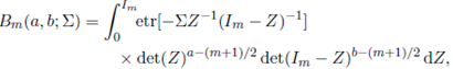 ()22
()22
where where Re(Σ) > 0 and a and b are arbitrary complex numbers. If Σ = 0, then Re(a) > (m − 1)/2 and Re(b) > (m − 1)/2.
3 Generalized extended matrix variate Gamma function
A matrix variate generalization of the generalized extended gamma function can be defined in the following way:
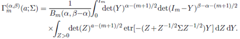
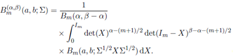
Definition 3.1. The generalized extended matrix variate gamma function, denoted by
Γm ( α,β ) a; Σ), is defined by
 ()23
()23
where Σ > 0 and a is an arbitrary complex number.
From the definition it is clear that for α = β, the generalized ex- tended matrix variate gamma function reduces to an extended matrix variate gamma function, i.e., Γ( α,α )(a; Σ) = Γ m (a; Σ). Further, if α = β and Σ = 0, then for Re(a) > (m− 1)/2, the generalized extended matrix variate gamma function reduces to the multivariate gamma function Γ m (a).
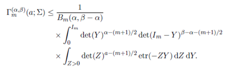
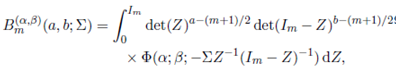
Replacing Φ(α; β; −Z − Z− 1 / 2Σ Z− 1 / 2) by its integral representation, namely,
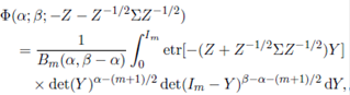 ()24
()24
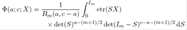
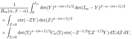
where Re(α) > (m−1)/2 and Re(β −α) > (m−1)/2, in (23), an alternative integral representation of the generalized extended matrix variate gamma function can be given as
 ()25
()25
Two special cases of (25) are worth mentioning. For m = 1, this expression simplifies to

Further, for Σ = Im
, substituting X = Y
1
/
2
ZY
1
/
2 with the Jacobian  in (25) and applying (21), the expression for
 is derived as
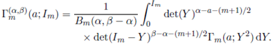 ()26
()26
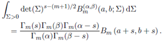
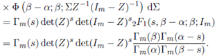
In the following theorem we establish a relationship between generalized extended gamma function of matrix argument and multivariate gamma function through an integral involving the generalized extended gamma function of matrix argument and zonal polynomials.
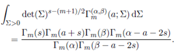
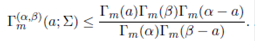
Theorem 3.1. For Re(s) > (m − 1)/2, Re(s + a) > (m − 1)/2, Re(α − a − 2s) > (m − 1)/2 and Re(β − a − 2s) > (m − 1)/2, we have
 ()27
()27
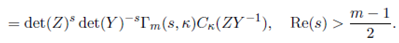
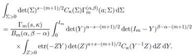
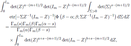
proof. Replacing Γ m ( α,β )(a; Σ) by its integral representation given in (25) and changing the order of integration, the left hand side integral in (27) is re-written as
 ()28
()28
where Re(α) > (m − 1)/2 and Re(β − α) > (m − 1)/2.
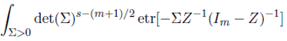
Further, using Lemma 2.1, the integral involving Σ is evaluated as
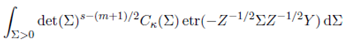
 ()29
()29
Replacing (29) in (28), to obtain
 ()30
()30
 Now, integration of Z using Lemma 2.1 yields the desired result.
Theorem 3.2. For a symmetric positive definite matrix T of order m, Re(s) > (m − 1)/2, Re(s + a) > (m − 1)/2, Re(α − a − 2s) > (m − 1)/2 and Re(β − a − 2s) > (m − 1)/2, we have
 ()31
()31
Corollary 3.2.1. For Re(s) > (m − 1)/2, Re(s + a) > (m − 1)/2, Re(α −a − 2s) > (m − 1)/2 and Re(β − a − 2s) > (m − 1)/2, we have
 ()32
()32
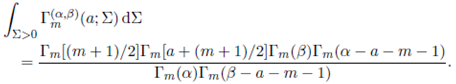
Note that the above corollary gives an interesting relationship between the generalized extended gamma function of matrix argument and multivariate gamma function. Substituting s = (m + 1)/2, in (32), we obtain
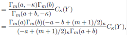
Theorem 3.3. For Re(s) > k 1 +(m− 1)/2 and Re(s+a) > k 1 +(m− 1)/2,
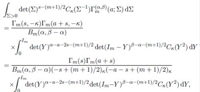 ()33
()33
where κ = (k 1 , . . . , km ), k 1 ≥ · · · ≥ km ≥ 0 and k 1 + · · · + km = k.
Proof. Replacing Γ m ( α,β )(a; Σ) by its integral representation given in (25), the left hand side integral in (33) is re-written as
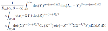 ()34
()34
Now, integrating first with respect to Σ and then with respect to Z by using Lemma 2.2, we obtain the desired result.
Theorem 3.4. For Σ > 0 and a > (m − 1)/2, α − a > (m − 1)/2 and
β − a > (m − 1)/2, we have
Proof. Let Z, Y and Σ be symmetric positive definite matrices of order m. Further, let λ 1 , . . . , λm be the characteristic roots of the matrix
Y 1 / 2 Z− 1 / 2Σ Z− 1 / 2 Y 1 / 2. Then

Since Z > 0, Y > 0 and Σ > 0, we have Y 1 / 2 Z− 1 / 2Σ Z− 1 / 2 Y 1 / 2 > 0, and therefore λ 1 + · · · + λm > 0. Further, as exp(−t) < 1, for all t > 0, we have
 () 35
() 35
Now, using the above inequality in (25), we have
 ()36
()36
Finally, integrating Z and Y by using multivariate gamma and multivariate beta integrals and simplifying the resulting expression, we obtain the desired result.
Theorem 3.5. Suppose that σ 1 and σn are the smallest and largest eigenvalues of the matrix Σ > 0. Then

Proof. Note that

and therefore
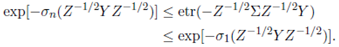
Now, applying the above inequality in (25), and using the integral representation of the generalized extended gamma function given in (25), we obtain the desired result.
By Hölder's inequality, it is possible to obtain an interesting inequality that follows.
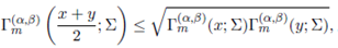
Theorem 3.6. Let 1 < p < ∞ and (1/p) + (1/q) = 1. Then, for Σ ≥ 0,
x > (m − 1)/2 and y > (m − 1)/2, we have
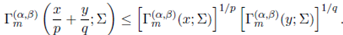 ()37
()37
Proof. Substituting a = x/p + y/q in (23) and using Hölder's inequality, we obtain the desired result.
Substituting p = q = 2 in (37), we obtain
where x > (m − 1)/2), y > (m − 1)/2, and Σ ≥ 0.
4 Generalized extended matrix variate Beta function
In this section, a matrix variate generalization of (6) is defined and several of its properties are studied.
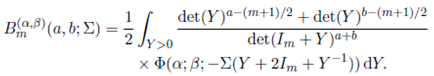
Definition 4.1. The generalized extended matrix variate beta function, denoted by Bm ( α,β )(a, b; Σ), is defined as
 ()38
()38
where a and b are arbitrary complex numbers and Σ > 0. If Σ = 0, then Re(a) > (m − 1)/2, Re(b) > (m − 1)/2.
Using Kummer's relation (16), the above expression can also be written
as
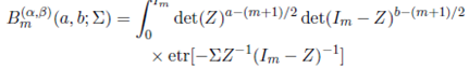
 ()39
()39
From (38), it is apparent that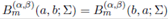 . Further,
  thereby
  is a function of the eigenvalues of the matrix Σ > 0.
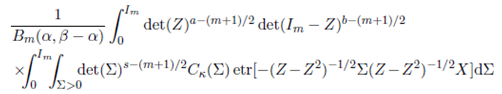
Replacing the confluent hypergeometric function by its integral repre- sentation in (38), changing the order of integration, and integrating Z by using (22), we obtain
 ()40
()40
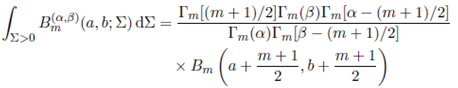
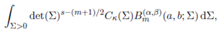
Theorem 4.1. For Re(s) > (m− 1)/2, Re(s + a) > (m− 1)/2, Re(s + b) > (m − 1)/2, Re(α − s) > (m − 1)/2 and Re(β − s) > (m − 1)/2,
 ()41
()41
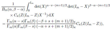
Proof. Replacing Bm ( α,β )(a, b; Σ) by its equivalent integral representation given in (39) and changing the order of integration, the integral in (41) is rewritten as
 ()42
()42
where we have used the result
Finally, evaluating (42) by using the definition of multivariate beta function, we obtain the desired result.
By letting s = (m + 1)/2, in (41), we obtain an interesting relation
between the multivariate beta function and the generalized extended beta function of matrix argument.
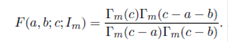
Theorem 4.2. For a and b arbitrary complex numbers and Re(Σ) > 0,
 ()43
()43
Proof. Substituting Z = (Im + Y ) − 1 Y with the Jacobian J(Z → Y ) = det(Im + Y ) − ( m +1) in (38), we obtain the desired result.
Theorem 4.3. For a and b arbitrary complex numbers and Re(Σ) > 0,
Proof. Noting that
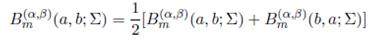
and substituting for Bm (α,β)(a, b; Σ) and Bm (α,β)(b, a; Σ) from (43), we obtain the desired result.
In the following theorem, we present an important inequality that shows how the extended matrix variate beta function decreases exponentially compared to the multivariate beta function.
Theorem 4.4. For Σ > 0, Re(α) > (m + 1)/2, Re(β − α) > (m − 1)/2, a > (m − 1)/2 and b > (m − 1)/2,
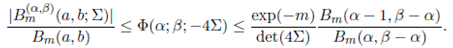
Proof. For Σ > 0, a > (m − 1)/2 and b > (m − 1)/2, Nagar, Roldán and Gupta 20 have shown that
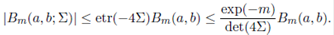
Now, using (40) and the above inequality, we obtain
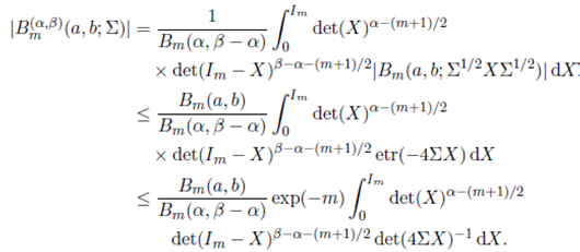
The desired result is now obtained by evaluating integrals using (14) and (9) and simplifying the resulting expression.
Theorem 4.5. Suppose that σ1 and σn are the smallest and largest eigenvalues of the matrix Σ. Then

Proof. Similar to the proof of Theorem 3.5.
The next result is obtained by applying the Minkowski inequality for determinants. The famous Minkowski inequality states that if A and B are symmetric positive definite matrices of order m, then

Theorem 4.6. For the generalized extended beta function of matrix argument, we have
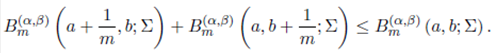
Proof. Replacing Bm ( α,β )(a + 1/m, b; Σ) and Bm ( α,β )(a, b +1/m; Σ) by their respective integral representation, one obtains
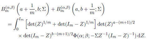
Now, by noting that det(Z)1 /m + det(Im −Z)1 /m ≤ 1 we obtain the desired result.
5 Results involving zonal polynomials
In this section, we will compute the integral
 ()44
()44
where Re(s) > (m− 1)/2, Re(s+a) > (m− 1)/2 and Re(s+b) > (m− 1)/2.
The calculation of this integral requires evaluation of the integrals of the form
 ()45
()45
where Re(a) > (m − 1)/2 and Re(b) > (m − 1)/2.
Recently, Nagar, Roldán-Correa and Gupta 20 have given computable representations of (45) for k = 1 and k = 2 which we state in the following three lemmas.
Lemma 5.1. For Re(a) > (m − 1)/2 and Re(b) > (m − 1)/2,
 ()46
()46
where
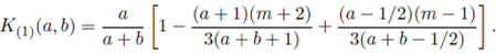
Proof. See Nagar, Roldán-Correa and Gupta 20.
Lemma 5.2. For Re(a) > (m − 1)/2 and Re(b) > (m − 1)/2,
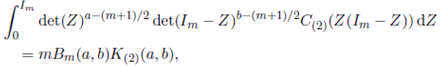 ()47
()47
Where
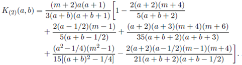
Proof. See Nagar, Roldán-Correa and Gupta 20.
Lemma 5.3. For Re(a) > (m − 1)/2 and Re(b) > (m − 1)/2,
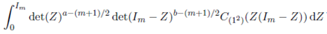
 ()48
()48
where
Proof. See Nagar, Roldán-Correa and Gupta 20.
In the following theorem and three corollaries we give closed form representations of the integral (44) for k = 1 and k = 2.
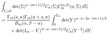
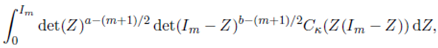
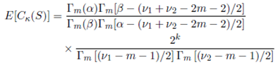
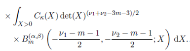
Theorem 5.1. For Re(s) > (m− 1)/2, Re(s + a) > (m− 1)/2, Re(s + b) > (m − 1)/2, Re(α − s) > k 1 + (m − 1)/2 and Re(β − s) > k 1 + (m − 1)/2,
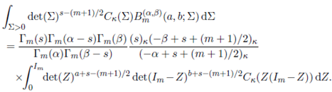 ()49
()49
Proof. Replacing Bm(α,β)(a, b; Σ) by its equivalent integral representation given in (40) and changing the order of integration, the integral in (49) is rewritten as
 ()50
()50
Now, evaluating the integral containing Σ using Lemma 2.1, we obtain

 (51)
(51)Further, substituting (51) in (50) and integrating with respect to X by using Lemma 2.4, we obtain
 ()52
()52
where Re(α − s) > k 1 + (m − 1)/2 and Re(β − s) > k 1 + (m − 1)/2. Now, substituting appropriately, we obtain the result.
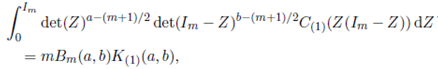
Corollary 5.1.1. For Re(s) > (m − 1)/2, Re(s + a) > (m − 1)/2 and Re(s + b) > (m − 1)/2,
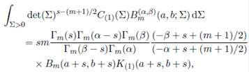 ()53
()53
where Re(α − s) > (m + 1)/2 and Re(β − s) > (m + 1)/2.
Proof. Substituting κ = (1) in (49) and using Lemma 5.1, we obtain the desired result.
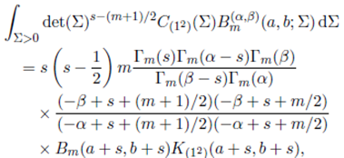
Corollary 5.1.2. For Re(s) > (m − 1)/2, Re(s + a) > (m − 1)/2 and Re(s + b) > (m − 1)/2,
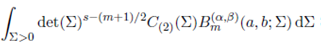
 ()54
()54
where Re(α − s) > (m + 3)/2 and Re(β − s) > (m + 3)/2.
Proof. Substituting κ = (2) in (49) and using Lemma 5.2, we obtain the desired result.
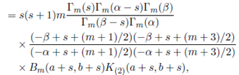
Corollary 5.1.3. For Re(s) > (m − 1)/2, Re(s + a) > (m − 1)/2 and Re(s + b) > (m − 1)/2,
 ()55
()55
where Re(α − s) > (m + 1)/2 and Re(β − s) > (m + 1)/2.
Proof. Substituting κ = (1, 1) in (49) and using Lemma 5.3, we obtain the desired result.
Corollary 5.1.4. For Re(s) > (m − 1)/2, Re(s + a) > (m − 1)/2 and Re(s + b) > (m− 1)/2, Re(α − s) > (m + 3)/2 and Re(β − s) > (m + 3)/2,
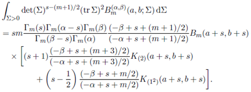
Proof. We obtain the desired result by summing (54) and (55) and using the result C(2)(Σ) + C(12)(Σ) = (tr Σ)2.
Corollary 5.1.5. For Re(s) > (m − 1)/2, Re(s + a) > (m − 1)/2 and Re(s+b) > (m−1)/2, Re(α−s) > (m+3)/2 and Re(β−s) > k1 +(m+3)/2,
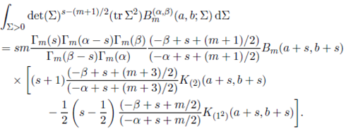
Proof. We obtain the desired result by using C(2)(Σ)−C(12) (Σ)/2 = (tr Σ2).
6 Application to multivariate statistics
The Wishart distribution, which is the distribution of the sample variance covariance matrix when sampling from a multivariate normal distribution, is an important distribution in multivariate statistival analysis. Recently, Bekker et al. (2, 3) and Bekker, Roux and Arashi (1) have used Wishart distribution in deriving a number of matrix variate distributions. Further, Bodnar, Mazur and Okhrin (5) have considered exact and approximate distribution of the product of a Wishart matrix and a Gaussian vector. The inverted Wishart distribution is widely used as a conjugate prior in Bayesian statistics (Iranmanesh et al. (14)). Knowledge of densities of functions of inverted Wishart matrices is useful for the implementation of several statistical procedures and in this regard we show that the distribution of the sum of dependent generalized inverted Wishart matrices can be written in terms generalized extended beta function of matrix argument. If  then its p.d.f. is given by
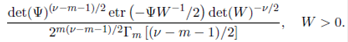
By replacing etr  by the confluent hypergeometric function of matrix argument
  and evaluating the normalizing constant, a generalization of the inverted Wishart distribution can be defined by the density
Further, a bi-matrix variate generalization of the above density can be defined as
 ()56
()56
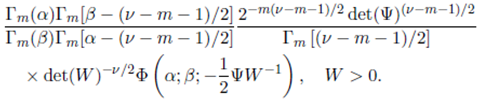
where W 1 > 0 and W 2 > 0. Note that if we take α = β in the above density, then W 1 and W 2 are independent, W 1 ∼ IWm (ν 1 , Ψ) and W 2 ∼ IWm (ν 2 , Ψ). Further, the marginal density of W1 is given by
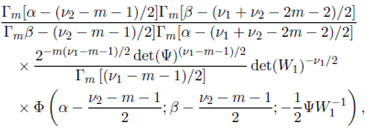 ()57
()57
where W 1 > 0. Likewise, the marginal density of W2 is given by
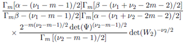 ()58
()58
where W 2 > 0.
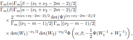
Theorem 6.1. Suppose that the joint density of the random matrices W 1 and W 2 is given by (56). Then, the p.d.f. of the sum W = W 1 + W 2 is derived as
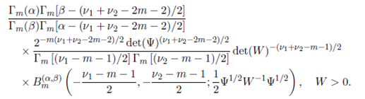
Proof. Transforming W = W 1 + W 2, R = W− 1 / 2 W 1 W− 1 / 2 with the Jacobian J (W 1 , W 2 → R, W ) = det(W )( m +1) / 2 in (56), the joint p.d.f. of R and W is obtained as
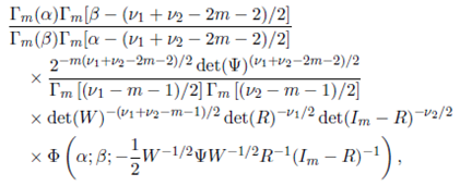
where W > 0 and 0 < R < Im. Now, integrating R by using (38), the marginal p.d.f. of W is obtained.
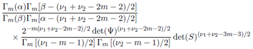
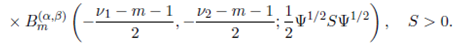
Corollary 6.1.1. Suppose that the joint density of the random matrices W 1 and W 2 is given by (56). Then, the p.d.f. of S = (W 1 + W 2) − 1 is given by
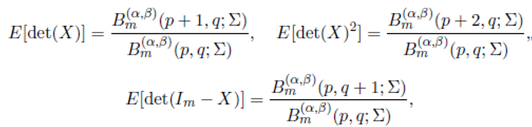
Next, we will derive results like E(C (1)(S)), E(C (2)(S)), E(C (12)(S)), E(tr S), E(tr S 2), E(tr S)2, E(S), E(S 2) and E(tr(S)S).
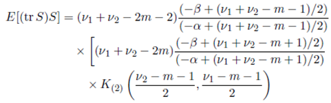
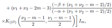
Theorem 6.2. Suppose that the joint density of the random matrices W 1 and W 2 is given by (56) with Ψ = Im and S = (W 1 + W 2) − 1 . Then
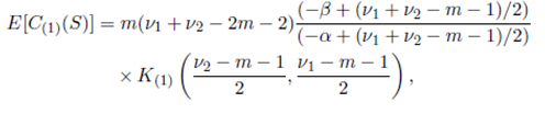
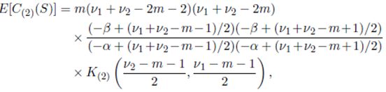
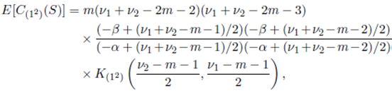
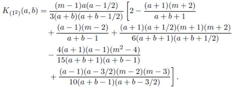
where K (1) , K (2) and K (12) are given in Lemma 5.1, Lemma 5.2 and Lemma 5.3, respectively.
Proof. The expected value of Cκ(S) is derived as
Now, setting s = (ν 1 + ν 2 − 2m − 2)/2, a = −(ν 1 − m − 1)/2, b = −(ν 2 −m− 1)/2 and using Corollary 5.1.1 for κ = (1), Corollary 5.1.2 for κ = (2), Corollary 5.1.3 for κ = (12), we obtain the desired result.
Theorem 6.3. Suppose that the joint density of the random matrices W 1 and W 2 is given by (56) with Ψ = Im and S = (W 1 + W 2) − 1 . Then
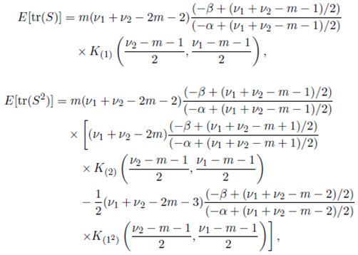
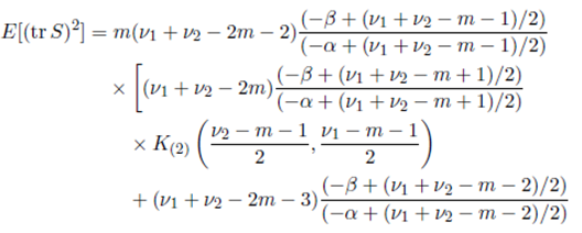
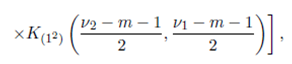
where K (1) , K (2) and K (12) are given in Lemma 5.1, Lemma 5.2 and Lemma 5.3, respectively.
Proof. We obtain the desired result by using C (1)(S) = tr(S), C (2)(S) − C(12)(S)/2 = (tr S 2) and C (2)(S) + C (12)(S) = (tr S)2, and Theorem 6.2.
Theorem 6.4. Suppose that the joint density of the random matrices W 1 and W 2 is given by (56) with Ψ = Im and S = (W 1 + W 2) − 1 . Then
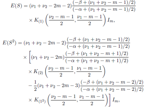
and
where K (1) , K (2) and K (12) are given in Lemma 5.1, Lemma 5.2 and Lemma 5.3, respectively.
Proof. Since, for any m × m orthogonal matrix H, the random matrices S and HSH' have the same distribution, we have E(S) = c 1 Im, E(S 2) = c 2 Im and E((tr S)S) = c 3 Im and hence E(tr S) = c 1 m, E(tr S 2) = c 2 m and E((tr S)2) = c 3 m. Thus, the coefficient of m in the expressions for E(tr S), E(tr S 2) and E((tr S)2) are c 1, c 2 and c 3, respectively. Finally, using Theorem 6.3, we obtain the desired result.
7 Generalized extended matrix variate Beta distribution
Recently, Nagar, Roldán-Correa and Gupta 20 and Nagar and Roldán-Correa 21, by using the integrand of the extended matrix variate beta function, generalized the conventional matrix variate beta distribution and studied several of its properties. We define the generalized extended matrix variate beta density as
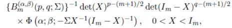
where −∞ < p < ∞, −∞ < q < ∞ and Σ > 0. If r and s are real numbers, then
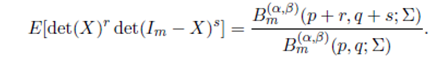
Specializing r and s in the above expression, we obtain