Inglês (pdf)
 Artigo em XML
 Referências do artigo
 Enviar este artigo por email
 Citado por SciELO
  Citado por Google
  Similares em
SciELO
Similares em
SciELO  Similares em Google
 Permalink
1 Introduction
The warehouse layout problem studies the design of storage or order picking areas of the warehouse 1. We focus on unit load warehouses with single command operations and U-flow configuration with parallel picking aisles. This means a unit-load warehouse with one pick and deposit (P&D) point 2. The warehouse layout problem in this context deals with finding the best position for the P&D point 3, determining the storage capacity location 4, designing the internal structure 5, sizing and dimensioning storage areas 6, establish aisle configuration 7),(8 and storage assignment policies 9.
We propose an optimization model to decide length and width of the warehouse and the location of the P&D to minimize the expected travel distance of picking or put-away operations. To this end, we use non-linear analytical models, as opposed to heuristics or simulation approaches commonly found in the literature. First, we develop a model assuming a random storage policy. Then, we extend the problem to consider a class-storage policy based on an ABC product classification.
In this paper, we gain insight into the warehouse dimensioning problem 6 under the most common storage assignment policy, the ABC classification 10 . Francis 3 developed the first attempt in warehouse dimensioning in a very simplified context and concluded for this context that a rectangular warehouse with one P&D should position it in the middle of its lower side. Bassan et al. 5 extends this work considering the detailed internal structure of the warehouse. On their model they do not propose a general conclusion about the length and width of the warehouse, the only consider specific situations. Also, they only faced the warehouse layout problem assuming a random storage policy which limits its application.
Afterwards, several papers work on that basis and integrate results with simulation approaches, heuristics 11 and metaheuristics as genetic algorithms and path relinking 12. According to Ballou 13, results suggests that warehouses should have a central P&D point and the warehouse should have a square shape. But this suggestions apply with very specific assumptions and those papers that study robust contexts use simulation and other non-optimal methods that do not allow to generate general conclusions. This is why, Gu at al. 6 state a need for research in the field that validates these models and extends their results.
In this paper, we focus on the most common case of class-based storage, the ABC product classification For ABC class-based storage, the optimal storage assignment policy is guaranteed and simple 14. It consists in locating the most important location in the most preferable position. Pohl et al. 15 label it as distance-based slotting strategy. In this way, class-based storage policies have a lower expected travel time to pick and retrieve loads when compared to randomize policies. Yu et al. 10 showed that even if the storage classes decrease the expected travel time, a small number of classes is optimal when a discrete number of items for each class is considered. Their results are robust to different kinds of ABC-demand profiles and warehouse shape. Guo et al. 16 extends this result by considering that each storage class introduced, also increases the space requirements of the warehouse. Storage locations are shared among less items. They found that the best design depends on the skewness of the demand profile and it effects the warehouse shape (relation between its width and length). Their analysis included the comparison of random, full turnover-based and class-based storage policies.
Thomas et al. 17) developed analytical expression to model the operations of put-away and order picking for the study of the warehouse configuration problem, which they defined as the warehouse shape and docks location. With this mathematical framework, Thomas et al. 18) proposed design guidelines for order picking warehouse including the ware- house shape, forward area size, and warehouse ceiling height. Authors validated their methods by means of industry data focusing on recommendations to decide if all docks of the warehouse should be located in one side, or there should be docks in both sides. Roodbergen et al. 19 propose a design method to simultaneously determine the routing policy, warehouse layout, and storage policy. The model demonstrates the impact of these control policies on the best configuration through a case study; however, no general guidelines were provided regarding the warehouse shape.
In the literature, there are some papers closely related with ours in the sense that they consider the warehouse layout problem jointly with storage assignment policies 15),(20),(21),(22. These studies approach the integrated problem using heuristics and simulation techniques and concluded that in general the best warehouse design under random storage policies also has a good performance for other storage assignments. The aim of this paper is to formalize, using an analytical point of view, this intuition that heuristics and simulation procedures suggest.
The paper is organized as follows: Section 2 presents an optimization model to minimize the expected travel time considering a class-based storage with an ABC product classification. Section 3 presents a robustness analysis. Finally, Section 4 presents possible applications of this analytical methodology and other findings of the paper for future research opportunities.
2 U-flow single command operations under class-based storage policy
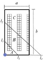
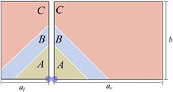
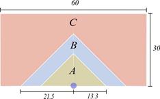
A common way to assign storage positions to products is to organize the available space following a class-based policy. In this paper we use an ABC product classification and a distance-based slotting strategy 15, locating the products with highest turnovers nearest to the P&D point (Figure 1). This section is devoted to find the best location for the P&D point and the optimal geometry for such a warehouse in order to minimize the Expected Value of the travel distance.
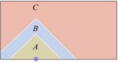
In Figure 1, we see that the A-products are located in the region nearest to the P&D point, as they are going to be the products with the highest probability to be selected. Farther away from the P&D point, we find the B- products that have medium turnovers. Finally, the C-products are located in the region farthest away from the P&D point. A-products region and B- products region have "triangular" shapes, because we are using a rectilinear distance 15.
The optimization process in this section is presented in two sections. First, in Section 2.1, we present a simplified model with the P&D point fixed to the lower left corner to find the optimal shape (a∗). Afterwards, in Section 2.2, we extend the model to include the position of the P&D point as a variable, p, and optimize it to find the optimal shape (a∗) and the optimal position of the P&D point (p∗).
2.1 Simplifted model with the P&D point ftxed on the corner
2.1.1 E ( D ) function We define the expected travel distance of the ware-house as the weighted average of the expected travel distance of the regions of the products.
The general equation of E(D) is
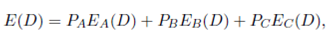 ()1
()1
where PA is the probability of selecting an item of A-products for a picking operation. The same definition applies for PB and PC . These probabilities are defined by the ABC product classification and depend on the demand of the products represented by tA, tB and tA, which is expressed in Equation (2a).
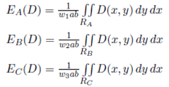
EA(D) is the expected travel distance for the region of A-products. The same definition applies for EB (D) and EC (D). Note that once we have established that an item belongs to a specific region, the probability of each point within the region is equal. Hence, we calculate the expected travel distance of each region (Equation (2b)) assuming a uniform probability within the region.
 ()2a
()2a
 (2b)
(2b)
where wi is the proportion of the area that each region occupies. Replacing Equations (2a)-(2b) into Equation (1), we have
 ()3
()3
Before we continue working on the expected travel distance, we are going to explain how to calculate tA, tB , tC , w 1, w 2 and w 3. Also, we define when an item located in position (x, y) belongs to the region RA, RB or RC .
Parameter ti, i = A, B, C, is the probability that the item of a picking operation j belongs to the i-th product group. And parameter wi, i = A, B, C, is the proportion of the area that i-th product group occupies.
We define that an item located in position (x, y) belongs to the region Ri for i = A, B, C, by establishing the boundaries of the regions and verifying if the item position belongs to the area defined by those boundaries.
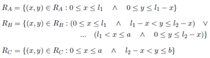
On the basis of Rao et al. 23, for the warehouse of Figure 2, we define the limits of the regions by means of two lines, y = l 1 − x, delimiting RA, and y = l 2 − x delimiting RB . RC is the region of the warehouse located in upper-side of y = l 2 − x. We define the functions of these limits as straight lines with slopes equal to one, because those are the "circles functions" in the rectilinear metric. That is, all points (x, y) > 0 that belong to the line y = l 1 − x are at the same distance to the P&D point.
We find l 1 and l 2 values setting up the area of RA to be equal to w 1 ab, the area of RB to be equal to w 2 ab and the area of RC to be equal to w 3 ab.
Therefore, we define the regions of the warehouse of Figure 2 by means of the polygons that enclose them in the following way.
Then, we use these limits in conjunction with Equation (3) to define an explicit expression for the expected travel distance of the warehouse of Figure 2.
 ()4
()4
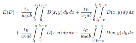
Equation (4) can not be used as the expected travel distance in general, because the polygons that enclose regions A, B and C vary depending on the values of a, b, l 1 and l 2.
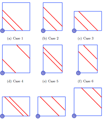
The boundary between two regions can start in two different sides (left and upper side) and finish in two others (right or lower side), giving rise to the four alternatives of Figure 3.
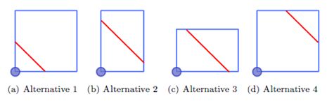
We need two boundaries for an ABC product classification, so all the combinations of the four alternatives need to be considered. It is left to the reader to verify that out of the sixteen theoretically possible combinations, there are three that are not feasible and four more that are redundant, leaving us with the nine cases presented in Figure 4.
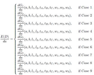
In summary, in order to establish a general function of the expected travel distance, we define E(D) by means of the following function of nine pieces, one for each case of Figure 4
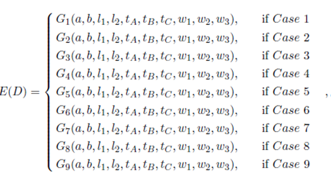 ()5
()5
where each  function is defined in appendix 5, and it is an expression similar to Equation (4).
2.1.2 Minimization of E(D) The optimization process of this section will find the best values for the main characteristics (a, b, l1 , l2) of a U- flow warehouse of area A, under class-based storage policy with an ABC product classification.
Model (6) will minimize function (5) under three constraint with variables (a, b, l1, l2) and (A, w1, w2, w3, tA, tB, tC ) as parameters. The first constraint guarantees that the area of the warehouse be the desired area. The second constraint sets the area of the region of A-products to be equal to the corresponding portion of the total area. The third constraint sets the area of the region of B-products to be equal to the corresponding portion of the total area.
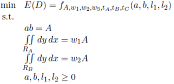 ()6
()6
This optimization problem has a non-linear objective function and three non-linear constraints. We simplify model (6) to obtain a model with only one variable and boundary constraints. This is achieved by means of the equality constraints. From each of the three constraints, we create a function of a that defines the variables b, l 1 and l 2.
Equation (7a) is directly derived from the first constraint. Equation (7b) defines li depending on the values of w 1, w 2, A and a. This function is based on the polygons used to delimit a region in Figure 3. The final outcome is that b = A/a, l 1 = g(w 1 , A, a) and l 2 = g(w 1 + w 2 , A, a).
 ()7a
()7a
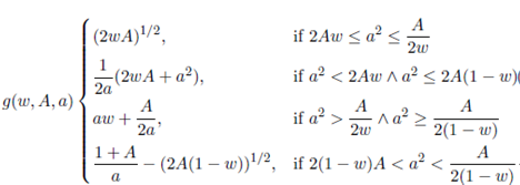 (7b)
(7b)
In this way, E(D) becomes a function depending exclusively on a.

 Min E(D) = ()8
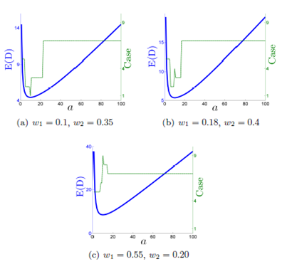
The objective function of the simplified model is a convex function. Figure 5 presents the plot of the objective function of model (8) for three warehouses with different values of w1 and w2. Each plot has two series, the first series, on the left axis, plots E(D) as a function of a. The second series on the right axis indicates the case of E(D) function (5) where it was evaluated. The optimal value of a in Figure 5(a) is achieved in Case 1, in Figure 5(b) is achieved in Case 4 and Figure 5(c) is achieved in Case 9.
 ()9
()9
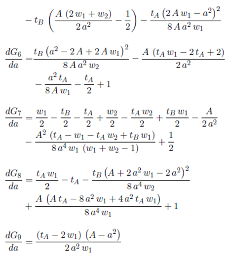
Now, we use the derivative of E(D) presented in Equation (9) to find the optimal value for a given the values of the parameters A, w 1, w 2, w 3, tA, tB and tC . Each piece of Equation (9) is defined in appendix 6. Now, we are going to find a function a∗ = h(A, w 1 , w 2 , w 3 , tA, tB, tC ) such that the derivative of E(D) (Equation (9)) evaluated in a∗ be equal to zero.
In Figure 5, we show that the optimal value is not always achieved in the same case. Hence, we create the function K(w 1 , w 2) (10) that establishes in which case the global minimum of E(D) is achieved given the value of the parameters A, w 1, w 2, w 3, tA, tB and tC .
From Equation (7b), we deduce that the case depends only on the values of A, w 1, w 2 and a. A is a constant that does not affect the optimization process and a is evaluated only in its optimal value, therefore the case only depends on w 1 and w 2. In Figure 6, we identify three regions: one in which the optimal value for a is achieved in Case 1, one in which the optimal value for a is achieved in Case 4, and one in which the optimal value for a is achieved in Case 9.
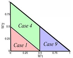
This means that if 0 ≤ w 1 ≤ 0.5 ∧ 0 ≤ w 2 ≤ 0.5 − w 1, E(D) will have its global minimum in Case 1 for all values of tA, tB, tC , a and A. The same applies for regions of Case 4 and Case 9. Therefore, this region definition is not for a specific example. These regions are defined in general and formally expressed as
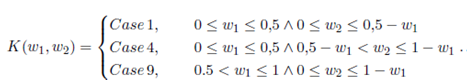 ()10
()10
Additionally, function (10) implies that regardless of the values of w1, w 2, w 3, tA, tB, tC , a and A, the global optimum of E(D) never is going to be achieved in Case 2, Case 3, Case 5, Case 6, Case 7 or Case 8. In consequences, we can ignore those cases in the optimization process.
Using K(w 1 , w 2), we create H(w 1 , w 2) = γ, a function with the derivative of E(D) in the cases where it reaches its global minimum.
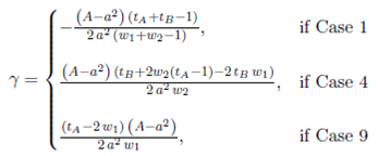 ()11
()11
In Equation (11), we see that a∗ = A 1 / 2 is the solution of H(w 1 , w 2) = 0 for any values of w 1 and w 2. Hence, a = A 1 / 2 is the value that minimize E(D) and this value is independent of the values of the parameters w 1, w 2, w 3, tA, tB and tC .
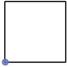
Figure 7: Optimal U-flow warehouse layout for the simplified model with an ABC product classification
Figure 7 shows the optimal U-flow warehouse layout when the warehouse has a class-based storage policy based on ABC product classification and the P&D point is fixed to the lower left corner. The most important result of this section is that shape of the optimal warehouse in this con- ditions is always a square, and it does not depend on the ABC product classification.
This is consistent with the cases that can be optimal (Cases 1, 4 and 9), which are the only cases with square shapes.
2.2 Model with an arbitrary position of the P&D point
Once we have developed a model with a fixed P&D point, in this section, we are going to extend that model to determine simultaneously the shape of the warehouse and the position of the P&D point that minimize the expected travel distance in a warehouse with an ABC product classification (Figure 1).
Next, we find the function of the expected travel distance of the ware- house in terms of the shape of the warehouse and the position of the P&D point. Then, we minimize the expected travel distance.
2.2.1 E(D) function In Figure 8, we represent a warehouse as the union of two split-warehouses obtained by a vertical cut in the position of the P&D point. This representation is useful because each split-warehouse has the P&D point on the corner, so we can use the E(D) function found in Section 2.1 to describe the expected travel distance of these split-warehouses. We
We define the expected travel distance of the total warehouse, ET (D), by the weighted average of the expected travel distance of its two split- warehouses as
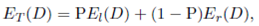 ()12
()12
where El(D) is the expected travel distance of the left split-warehouse, Er(D) is the expected travel distance of the right split-warehouse and P is the proportion of travels that pickup or deposit an item on the left split-warehouse.
It is worth to mention that, in this section, labels a, p, A, tA, tB, tC, w1, w2, and w3 have the same meaning as in Section 2.1.
The proportion P is defined as
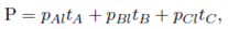 () 13
() 13
where pAl is the proportion of area of A-products region that is in the left split-warehouse. The same definition applies for pBl and pCl.
We use Equation (4) to define El(D) and Er(D) as
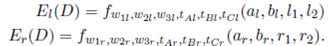 ()14
()14
where 

Note that, the parameters of w1l, w2l, w3l, tAl, tBl and tCl, are not the same as those of the total warehouse w1, w2, w3, tA, tB and tC . The folowing equation shows how to calculate these parameters for both split- warehouses
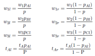
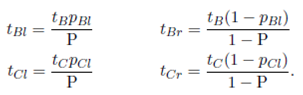
We label zl(a, p) to  (pa, A/a, g(w1l, pA, pa), g(w1l
+ w2l, pA, pa)) and zr
(a, p) to
(pa, A/a, g(w1l, pA, pa), g(w1l
+ w2l, pA, pa)) and zr
(a, p) to  (pa, A/a, g(w1r, pA, pa), g(w1r
+ w2r, pA, pa)). Afterwards, we rewrite Equation (14) in terms of zl
(a, p) and zr
(a, 1 − p). Therefore, El
(D) = zl
(a, p) and Er
(D) = zr
(a, 1 − p). By replacing those functions in Equation (12), we obtain
(pa, A/a, g(w1r, pA, pa), g(w1r
+ w2r, pA, pa)). Afterwards, we rewrite Equation (14) in terms of zl
(a, p) and zr
(a, 1 − p). Therefore, El
(D) = zl
(a, p) and Er
(D) = zr
(a, 1 − p). By replacing those functions in Equation (12), we obtain
 ()15
()15
Note that in the definition of the proportion P of Equation (13), the parameters pAl, pBl and pCl depends on the width and area of the left split-warehouse. In general, we define Pas  . We label
  and obtain
Finally, we replace  in Equation (15) and have
 ()16
()16
2.2.2 Minimization of E(D) In Section 2.1.2, we showed that the best shape for a warehouse with the P&D point in the corner is a square, regardless of the ABC classification of the products. Using this fact, in this section, we show that the P&D point should be located in the middle of the width of the warehouse (p = 1/2) and the best shape for the warehouse is a = 2b, without regard to the ABC product classification.
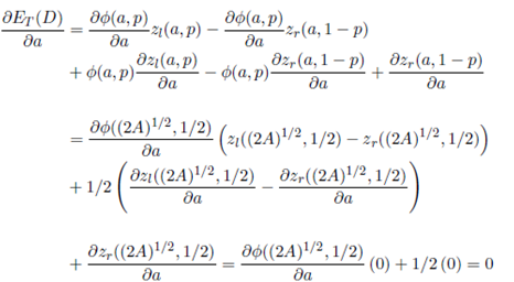
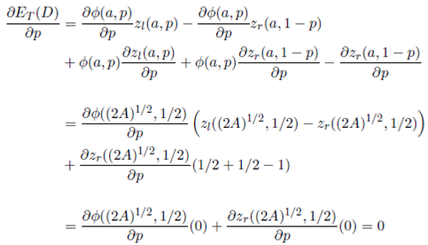
The global minimum of ET (D) (Equation (16)) is the solution of the following system of Equations
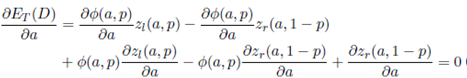 ()17a
()17a
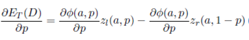
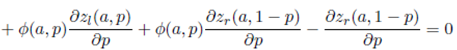 (17b)
(17b)
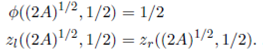
In the following, we solve the system of equations (17) to obtain the solution p∗ = 1/2 and a∗ = (2A)1/2 .
Note that in Section 2.1, we prove that the best shape of a warehouse with a fixed P&D point is a square and in this context that means that
 ()18
()18
Furthermore, when p∗ = 1/2 and a∗ = (2A)1 / 2 the warehouse is symmetric and that means two things. First, the proportion of total travels that goes to the left split-warehouse is 1/2. Second, the expected travel distance for both split-warehouses is the same. Therefore,
 ()19
()19
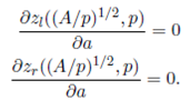
In the following equations, we use Equations (18)-(19) to show how
p = 1/2 and a = (2A)1/2 make that  and
and  .
.
Finally, we find the optimal value of b from the fact that A = ab. Hence, b = (A/2)1/2 and a = 2b, as it was proposed at the beginning of this section.
This result is consistent with the one obtained in Section 2.1.2. We proved that the best shape for a warehouse with the P&D point in the corner is a square. And in this section, we show that the total warehouse is composed by two split warehouses with square shape.
In conclusion, in U-flow single command warehouses under a class-based storage policy with an ABC product classification, the width of the warehouse should be twice its length regardless of the ABC product classification and the P&D point should be in the middle of the width of the warehouse
(Figure 9). It is worth to mentioning that these results are equal to the ones obtained with a random storage policy.
3 Robustness analysis
In an industrial environment, it is not always possible to build a warehouse with optimal characteristics. We want to provide a technical argument that helps warehouse planners to decide how much deviation from the optimum is acceptable.
With the optimal model of Section 2.2.2, we want to determine how important it is to select the optimal values for a and p. That is, how critical is a certain deviation from the optimum values of the warehouse dimensions and location of the P&D point.
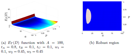
Figure 10(a) shows the plot of ET (D) as function of a and p for a warehouse with fixed values of A, tA, tB, tC , w1, w2 and w3. From the shape of ET (D), we see that it has a unique optimum point and a very flat region around it. In Figure 10(b), we show the robust region in light colour defined as the points (a, p) such that ET (D) is greater than the minimum in at most five percent.
We see that having a∗ constant, we can increase or decrease p up to 50% from p∗ without making ET (D) increase more than five percent over its minimum value.
Moreover, we see that having p∗ constant, we can increase or decrease a up to 20% from a∗ without making ET (D) increase more than five percent over its minimum value.
Having this robust region implies that warehouse planners have some range of flexibility to choose a and p. Also, it states that it is more important to be accurate with the value of a than with the value of p.
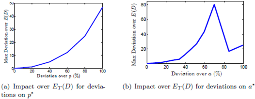
In Figure 11, we present the robustness analysis over a simulation of 100.000 cases where we vary values of A, w1, w2 and w3. In Figure 11(a), we show the maximum deviation over ET (D) for a deviation on p∗. We can see that ET (D) increase at most 5% over its minimum for a deviation of 40% around p∗. In Figure 11(b), we show the maximum deviation over ET (D) for a deviation on a∗. We can see that ET (D) increase at most 12% over its minimum for a deviation of 40% around a∗.
In conclusion, it is not critical to select the precisely optimal values. If there is a technical reason that suggests to implement a non optimal shape and position of the P&D point, there exists a neighborhood of solutions for which the deviation from the optimal expected travel distance will be relatively small.
4 Conclusions and Future Research
In this paper, the authors analysed U-flow warehouses under class-based storage policy with an ABC product classification.
We presented a model for U-flow warehouses under class-based storage policy with an ABC product classification. With this model, we concluded that in a warehouse under class-based storage policy with an ABC product classification and a fixed P&D point located in a lower corner, the best shape for the warehouse is a square.
When we treat the position of the P&D point as a variable, we obtain the same results than when we assume a random distribution: the P&D point should be located in the middle of the width of the warehouse and the width of the warehouse should be twice its length. In Section 3, we analysed the robustness of the function of the expected travel distance and, as we obtained assuming a random distribution, the function is flat around its optimal point (Figure 11).
The most important contribution of this paper is that we mathematically proved that it does not matter if the distribution of the products is assumed to be random or represented by any ABC product classification, the best shape for a U-flow single command warehouse under class-based storage policy is a rectangle with a width twice its length and the P&D point should be located in the middle of the width of the warehouse.
For future research, we recommend to extend this model to determine if it is possible that in a rectangular warehouse with other storage policies, the best position for the P&D point is always the middle of the width of the warehouse. Also to establish when the distribution of the products will change the optimal shape we found for the ABC product classification.
Finally, flow-through warehouses (such as pure cross-docking operations) can be studied using the analytical methodology presented here. Aspects such as number of available docks, timing of arrivals and departures, number of resources available or required could be used to determine the most efficient configurations of the warehouse and the temporary needs for storage (if any) when operations are not perfectly synchronised due to constraints in the use of resources.