


 English (pdf)
 Article in xml format
 Article references
 Send this article by e-mail
 Cited by SciELO
  Cited by Google
  Similars in
SciELO
Similars in
SciELO  Similars in Google
 Permalink
1 Introduction
Currently, there are around 870 million automobiles in the world. This makes the road infrastructure of some overpopulated cities is not sufficient with respect to the great demand, collapsing in huge traffic jams, generating chaos and plunging the humankind into one of the most increasing problems like traffic congestion [1].
Although, automobiles represent a solution to the mobility problem, they constitute one of the major sources of pollution. Due to this supply a series of toxic substances in the environment, well known as greenhouse gases (carbon monoxides CO, hydrocarbons, among others), as a consequence of the complete non-combustion of the petroleum products necessary for the functioning of cars. In the same way, the produced noise pollution may generate a series of negative responses in human beings, such as balance disorders, ill feeling and fatigue, among others. On the other hand, the consequences caused by traffic accidents add invaluable losses because these take the lives of 1.2 million people in the world and more than 50 million individuals are injured [2],[3],[4].
Due to the vehicular problems in the cities, there is a need to carry out theoretical studies [5],[6]. This is why it is daily invested in time, human capital and development of new theories or even creation of tools that provide scientific basis to the possible strategies implemented by the government entities to improve mobility in cities. As an example, and to mention one of the most relevant authors in literature, as can be seen in Toledo [7],[8],[9], the construction of a model in which one single vehicle is considered, moving through a twoway traffic light sequence, with a specific period; the most relevant contribution of this work, is that the nontrivial dynamics depends on the finite acceleration and breaking power of vehicles for a set of parameters.
In a later work, Toledo establishes in [10], control strategies based on the synchronization of the traffic lights, which allowed to improve the vehicle traffic, moreover, the resonance in terms of travel time, speed and fuel consumption were studied in this work. An important result of the Toledo model, apply the control strategy, is that the behavior close to resonance does not depend on finite acceleration and breaking power of the vehicle. Furthermore, in this deterministic model, it was shown that the resonance was an independent universal behavior of the geometry of the system for the case of the green wave strategies.
In 2009, Varas researched whether the universal behavior close to resonance persists, when several cars interact along the same route. To know the behavior of this dynamics, used a cellular automaton model [11] . One of the most recent works in this respect, is the work carried out by Mesa in [12], where the description and comparison of four vehicle traffic models are presented. This work explains the dynamic of one single car that moves through a sequence of traffic lights that turns on and off. See more on [13],[14].
The mathematical model, as well as the results of the numerical analysis are presented in this document. The main contribution, which is intended to be highlighted on this occasion, is quite useful at the moment of analyzing the periodic behaviors associated with the dynamic of the vehicle. Thus, the methodology used is explained to carry out the stability analysis and consequently, conclude about how the orbits in question are or are not stable. This in order to propose a formula that allows to calculate the fuel consumption, if necessary, a vehicle had one dynamic or another.
2 Mathematical model
In the Toledo’s one-dimensional model [7], it is assumed that an automobile travels through a two-way (green and red) traffic light sequence, where the car presents one of the following behaviors:
Positive acceleration a − until the vehicle reaches the cruising speed or maximum speed v max .
Constant speed v max , when the acceleration is zero.
Deceleration −a − until the vehicle stops.
A zero speed when the vehicle is stationary, waiting for the traffic light to turn green
2.1 Description of the model
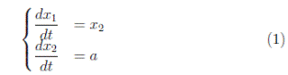
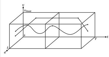
From the above and [8], the dynamic of the system can be represented using a piecewise soft system, four situations are presented in this model, which depend on acceleration, that is, accelerated state, zero state with maximum speed, zero state with zero speed and decelerated state. To make an appropriate description of each event, it is considered that the following state variables (x 1 , y 1) are the position and velocity of the vehicle respectively, a acceleration of the vehicle in a time t, which will change depending on which state the vehicle is:
2.2 Conftguration of the traffic light
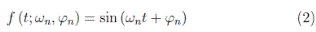
It is considered that the nth traffic light will be modelled through the function (2).
Where
ω n =
: indicates the switching frequency of the nth traffic light.
T n : the cycle of the nth traffic light, i.e., the time that the green light takes to turn green again.
ϕ n : denotes the phase difference between traffic lights.
Moreover, these are the following assumptions or conditions that should be complied by the traffic lights:
If sin (ω n t + ϕ n ) > 0, then the traffic light is green.
If sin (ω n t + ϕ n ) > 0, then the traffic light is red.
The normalized cycle T sn of the nth traffic light was used in [2],[3]. It is necessary to highlight the importance of the Equation (3), given that this allows to obtain the real cycle of the nth traffic light in units of time, making use of the system parameters.
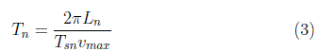
where L n is defined as the distance that separates one traffic light from another and v max the maximum velocity, whose conclusion may be; the cycle of the nth traffic light is obtained in units of time.
2.3 Dynamic system states
Making use of the system of Equation (1) and the traffic light conditions, it is established that each dynamic state can be expressed in the following way:
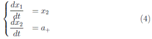
2.4 Accelerated state “ S +”:
it occurs when the driver increases the speed constantly, i.e., the car has a constant and positive acceleration a + , until the vehicle reaches the cruised speed v max owed on the road. In this way, the system is as follows in the Equation (4).
2.5 Zero state:
this is because the car may present zero acceleration in two situations during the tour. For this reason, the zero state is divided into two modes:
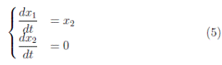
2.5.1 Zero state with maximum speed “ S 0m ”: it occurs when the vehicle reaches maximum speed allowed on the road v max . For this reason, this velocity should be maintained, i.e., its acceleration is zero. Later, the system of equations is determined by the Equation (5).
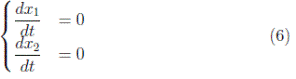
2.5.2 Zero state with zero speed “ S 0”: it occurs when the vehicle is stationary, considering the position of a traffic light, which is expected to turn green, i.e., sin (ω n t + ϕ n ) > 0,. Then, the system of equations is as we shown in (6).
2.6 Decelerated state “ S − ”:
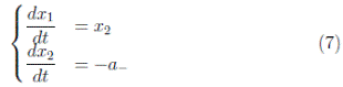
when the evolution of the system is in a decelerated motion, the vehicle is forced to decrease its velocity constantly, due to the traffic light is red, i.e., sin (ω n t + ϕ n ) 0. Then, the equations associated with this state are those found in Equation (7).
When the vehicle approaches the nth traffic light with speed x
2, the driver should decide whether to slow the car down or not, depending on the following traffic light signal. Then, the safety distance or stopping distance is defined as the distance required by a car that travels at a velocity x
2 to stop. Determining the safety distance is necessary to optimize safety in vehicles, line of tracks and signaling design [12]. For this case,
 is defined as the safety distance [7],[8].
3 Simulation analysis
In [8], the behavior of a vehicle was studied when it is considered that all the traffic lights present fixed distances and have the same switching rate with a zero phase difference; i.e., L n = L, ω n = ω and ϕ n =0 respectively, different types of orbits were obtained under these assumptions. The main objective of this article is to study the stability of the periodic orbits 1T and 2T as a particular case, as well as fuel consumption, assuming that this is proportional to the mechanical energy. In addition to carry out the respective comparisons in the cases in which the dynamics of the vehicle evolves through a green wave and the periodic orbits 1T and 2T .
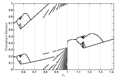
3.1 Bifurcation diagram
Assuming the fact that L n = L, ω n = ω and ϕ n = 0, a bifurcation diagram was built, see Figure 1, this was developed varying the normalized traffic light cycle. For the equation (3) and the assumptions previously described, it is assumed that T sn = T s , the equivalence illustrates that this parameter will be the same for all the traffic lights, this is charted along the horizontal axis and the normalized position of the car is shown in the vertical axis. Different phenomena can be observed in this bifurcation diagram, indicating the dynamic richness of the system; with behaviors such as fractals, multiple periods, duplicity of period, chaos, hard and soft bifurcations, among others.
In Figure 1 Bifurcation diagram, when T s takes values between 0.7 and 1, lines that increase are observed as T s approaches to the value of 1 and multiple periods are observed. Then, when T s is increasing, it presents a duplicity of period route to the chaos, where this chaotic behavior is truncated and an orbit from period two appears again and finally, an orbit form period one. It is important to highlight that hard and soft transitions are also observed in Figure 1. For example, there is a soft transition when 1.0 < T s < 1.1 and a hard transition is observed when 1.3 < T s < 1.4.
3.2 Evolution in time
Before observing the charts that show state variable evolution, it is important to highlight Table 1, given that it relates the normalized parameter cycle T _s with the cycle T _n and the time in green of a traffic light using the Equation (3), where the parameters are v max = 14m/s and L = 200m. In addition to the function presented in the Equation (2), which models the traffic light, it is assumed that the positive semi cycle is equal to the negative semi cycle, therefore, the time in green is equal to the time in red.
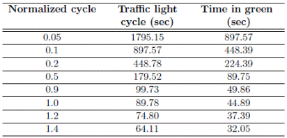
As observed in Table 1, when T s is close to zero, the time in green from the traffic light is long. For example: for T s = 0.05, the time in green is approximately 15 minutes, which would make no sense to configure a traffic light with a cycle T n = 30 mins. Therefore, the orbits for T s = 1.4, T 2 = 1.2 and T s = 1.0 were obtained in [8]. The normalized speed of the vehicle is shown in a thick continuous line, the normalized position is shown in a dashed line and the traffic light signal is shown in a thin continuous line, that allow to evidence different behaviors for each value used from the parameter are shown in Figures 2, 3 and 4.
Comparing the bifurcation diagram from Figure 1 with the results in Figure 2, it is assumed that an orbit of period one is observed in this case. Moreover, with the help of the circle from Figure 2, which allows to visualize the normalized position of the vehicle when the traffic light switches. It is important to highlight that the position is always the same.
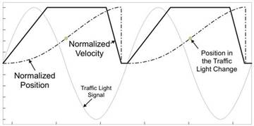
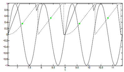
Figure 3 Evolution in Time for T s = 1.2 Simulation. The dotted line refers to the normalized position, the solid dark line refers to the normalized speed, the green circular point refers to the signal change at the traffic light, and the sine signal is the periodic behavior that represents the ignition frequency and off for the traffic light. Source: The authors.
In Figure 3, an orbit from period two is observed when the normalized traffic light cycle takes the value of T s = 1.2. Furthermore, the circles show the normalized position of the car when the traffic light changes from green to red, given that the sine function changes the positive semi cycle to negative and this coincides every two traffic lights; in addition, the vehicle is required to stop every two traffic lights.
In Figure 4, the thick continuous line remains at its maximum value; i.e., the vehicle maintains its maximum speed and achieves to cross all the traffic lights in green, this behavior is known as a green wave. These charts were obtained and analyzed in [12].
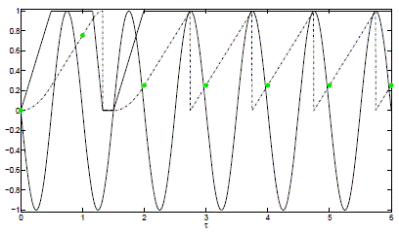
Figure 4 Evolution in Time for T s = 1.0 Simulation. The dotted line refers to the normalized position, the solid dark line refers to the normalized speed, the green circular point refers to the signal change at the traffic light, and the sine signal is the periodic behavior that represents the ignition frequency and off for the traffic light. Source: The authors.
4 Stability analysis
A stability analysis for a periodic orbit 1T and a periodic orbit 2T will be carried out in this section. These orbits were found in [8] for the model that describes the dynamic of a single car that travels on a road, which has n traffic lights, where it was considered that all the traffic lights present fixed distances, i.e., L n = L. The function modeled by the traffic light is given by the Equation (2), with ω n=ω , in this way, they have the same cycle T and a zero-phase difference, ϕ n = 0. This indicates that all the traffic lights have the same frequency, the switching frequency.
The Figure 5 explains the visualization of the model solution space. Due to the periodicity of the solutions in Figure 2, the X-axis represents the distance traveled by the vehicle. This takes values in the interval
 , where L is the distance between two consecutive traffic lights; time t is illustrated along the Y-axis. This variable takes values in the interval
 , where T is the traffic light cycle. Finally, the Z-axis represents the velocity v of the car, which takes values in the interval
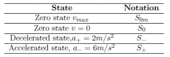
 . To represent the orbits to be studied, the notation explained in Table 2 will be adopted, which will depend on the state of the vehicle:
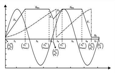
4.1 Periodic orbit 1T
The Figure 6 is obtained using Figure 2 and notation form Table
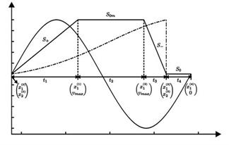
First of all, it is important to explain the notation used in Figure 6:
x 1 (i) : the final position in the i-th stretch
x 1 (i) : the final velocity in the i-th stretch
x 2 (0): initial position of the path
x 2 (0): initial velocity of the path.
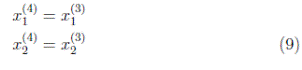
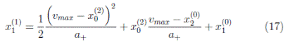
Where i = 1, 2, 3, 4. In addition, a stretch is considered as a part of the path, in which a state is conserved. For example, the first stretch in Figure 6 begins when the vehicle presents a position x 1 (0) and a speed x 2 (0) and finishes when the vehicle has a maximum speed v max and is in position x 1 (1).In this way, the periodic orbit 1T has four stretches, given that four changes of state occur.
As the interest of this section is to study the stability of the orbit 1T s+s oms−s0 , it is necessary to find the Jacobian matrix:
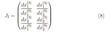
To find each component of J 1, Figure 6 is used as well as the Equations. (4), (5), (6) and (7).
By observing Figure 6, it is understood that in the fourth stretch, the car is in zero state S 0, that is, the vehicle is stationary, therefore:
To determine these unknown numbers, it is necessary to know the final position and velocity of each stretch.
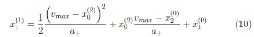
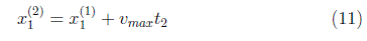
the final position x 1 (2) of the second section is:
Where
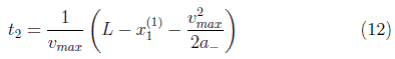
and substituting x 1 (1), the travel time from the second stretch is determined as:
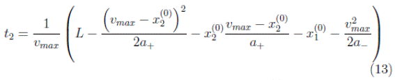
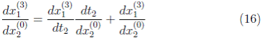
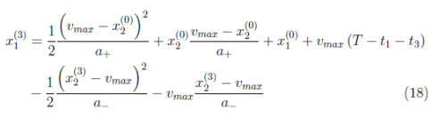
Finally, it is assumed that the final position x 1 (3) in the third stretch is given by:
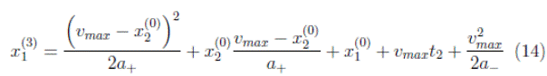
In addition, by observing Figure 6, it is assumed that the car stopped when finishing the third stretch, then the final speed in the third stretch is x
2
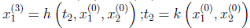
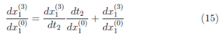
(3) = 0. To find the first order partial derivative, the Equations. (13) and (14) are used, it also should be considered that:
 , therefore:
In the same way,
 is found as follows:
Then, calculating the respective derivatives, it is understood that the Jacobian matrix J 1 is the zero matrix. Therefore, it has two associated zero eigenvalues. According to [15], if the product of the eigenvalues is zero in the case of a dimensional M map, this means that the orbit 1T S+S omS−S0 is extremely stable [16],[17].
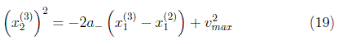
4.2 Periodic orbit 2T
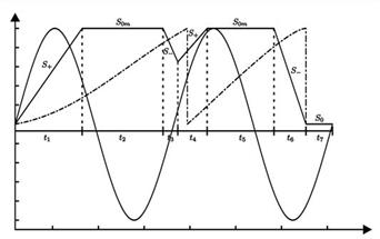
Figure 7 is obtained using Figure 3 and notation form Table 2, this is a graphic representation for the periodic orbit 2T for the model.
From Figure 7 and making use of Table 2, the map that allows to study the periodic orbit 2T is denoted as 2T S +SomS−SomS−S0 .
It should be remembered that:
x 1 (i) : the final position in the i − th stretch. x 2 (i) : the final velocity in the i − th stretch.
Where i = 1, 2, 3, 4, 5, 6, 7.
The periodic orbit 2T has seven stretches, given that seven changes of state occur. As previously in the periodic orbit 1T, in this way it is necessary to determine the final position and speed in the seventh stretch x 1 (7) and x 2 (7) respectively, in terms of the initial conditions x 1 (0)
and x 2 (0); for this, it is necessary to use the equations. (4), (5), (6) and (7), in order to find the final position and speed of each stretch.
The final position in the first stretch is given by:
For the third stretch of the travel, the final position x 1 (3) in terms of the initial conditions is:
In the same way, the final speed x 2 (3), in the same stretch, is determined by:
Given that the work is being done with a periodic orbit 2T and with help of Figure 7, it is assumed that:
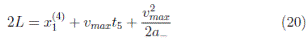
Then, the travel time in the fifth stretch t 5 is given by:
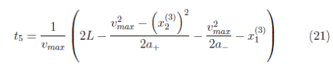
Finally, in the sixth stretch, the final position x 1 (6) = x 1 (7) is determined by:
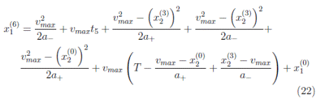
The purpose is to determine the stability of orbit 2T S +SomS−S+SomS−S0 , for this it is necessary to find the Jacobian matrix as follow:
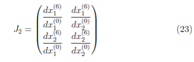
From the previous, the Jacobian matrix J 2 is determined as:
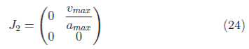
Hence, the Jacobian matrix J_2 has two zero eigenvalues, then its product is zero and for the stability criterion for dimensional M maps, it is understood that the orbit 2T S +SomS−SomS−S0 is extremely stable [16],[18].
5 Fuel consumption
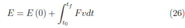
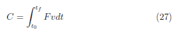
For this work, it is assumed that the car moves on a straight path, being subjected to an acceleration or deceleration, both constants, reason why the weather conditions will not be considered. The fuel consumption calculation will be especially made for the periodic orbits 1T and 2T and finally for the green wave. In first place, the instantaneous power P is considered as the energy transfer portion E in time t [19]
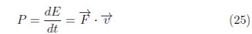
Where:
t f : final time of the stretch t 0: initial time of the stretch. F: the force vector module.
v: the velocity vector module.
t: time.
According to [10], fuel consumption C can be estimated as shown in the Equation (27).
It is important to clarify that the friction force F r will be considered, which is opposite to movement, external forces such as aerodynamic drag will not be considered, and the energy spent due to internal frictions in the mechanism of the vehicle is also omitted. The dissipation sources in the vehicle movement, which will depend on the state of the car (accelerated, zero and decelerated) will be described below. To represent the states of the vehicle, the notation explained above and summarized in Table 2 will be adapted.
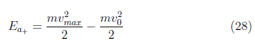
Accelerated state “ S + ”: when the vehicle begins the route with initial speed v 0 and the driver accelerates until reaching the permissible maximum or cruising speed on the route, the kinetic energy shift is calculated in Equation (28).
Zero State with Maximum Speed “ S 0m ”: when the vehicle travels a distance x r free of stops, the work carried out is opposed to the friction force and assuming a constant coefficient of friction μ along the road, we have the following Equation (29).

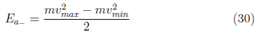
Decelerated State “ S − ”: when the vehicle travels with a maximum speed until reaching the safety distance and the traffic light is red, so the driver is obliged to slow down until reaching the minimum speed v min ; therefore, the energy lost while decelerating is given by the Equation (30).
Zero State with Zero Speed “ S 0”: when the vehicle is stationary, considering the position of a traffic light, which is expected to turn green, the idle fuel consumption C 0. The vehicle is stationary when it is in zero state, then fuel consumption is proportional to awaiting time with respect to the traffic light, i.e., C 0 = k t e , where t e is the time waited by the driver until the traffic light turns green and k is the constant of proportionality.
With the above, fuel consumption is calculated for the cases where it displays a behavior for the periodic orbits 1T and 2T and the green wave for the model already explained.
5.1 Fuel consumption for a periodic orbit 1T
The graphic representation of the periodic orbit 1T is observed in Figure 8, in which four changes of state occur, these are: accelerated S +, zero with maximum speed S 0m , decelerated S − and zero with zero speed S 0.
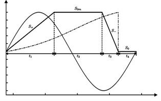
The fuel consumption of the vehicle applied to the orbit 1T S +SomS−S0 will be carried out through each state, applying any of the Equations. (28), (29) or (30).
For this orbit, it is necessary to calculate the consumption in each state and add them algebraically. In this way, an approximation of fuel consumption between two consecutive traffic lights is obtained. When multiplying the value found by the number of stretches n 1, the total of the fuel used during the travel will be obtained, where n is the number of traffic lights. In addition, it is considered that a stretch is the path between two consecutive traffic lights.
From the above, it is assumed that the total fuel consumption between two consecutive traffic lights is the sum of the consumption in each state, i.e.:

As the waiting time with respect to the traffic light is small in comparison with the travel time, it is assumed that the fuel consumption will be zero, i.e., C 0 ≈ 0. Therefore, the consumption is:
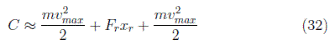
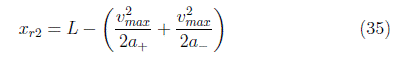
Where the distance traveled by the vehicle without stopping is:

And the distance traveled in the accelerate state S + is:
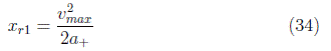
The distance traveled in the zero state with maximum speed S 0m is:
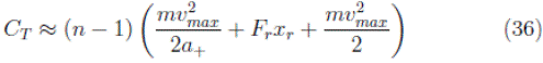
As the purpose is to find the fuel consumption used during the travel through the sequence of n traffic lights for the periodic orbit 1T , then the Equation (32) is multiplied by the number of stretches n − 1.
Then, the total fuel consumption throughout the travel is given by:
5.2 Fuel Consumption for a Periodic Orbit 2T
The graphic representation of the periodic orbit 2T is observed in Figure 9.
To calculate the fuel consumption of the vehicle using the periodic orbit 2T S +SomS−S+SomS−S0 , it will be made again through the states. For this case, it is necessary to calculate the consumption in each state and add it. In this way, an approximation of the fuel consumption between three consecutive traffic lights would be obtained. Seven changes of states of the vehicle occur for the periodic orbit 2T , the terms explained for the periodic orbit 1T will be used to calculate the fuel consumption in each state.
As the objective is to find an expression that represents the fuel consumption throughout the travel through the sequence of n traffic lights for the periodic orbit 2T , it should be considered that a car completes a stretch when it has passed three consecutive traffic lights, and this makes that the general expression of fuel consumption for this periodic orbit 2T depends on whether the number n of traffic lights is even or odd.
When the number of traffic lights is odd, i.e., n = 2k +1 where k is the number of stretches, then the total fuel consumption is expressed as:
Now, n can be expressed in the following way is even: n = (2k +1) + 1 where k is the number of stretches, then the total fuel consumption is expressed as:
5.3 Fuel consumption for the green wave
The graphic representation of the green wave is observed in Figure 10.
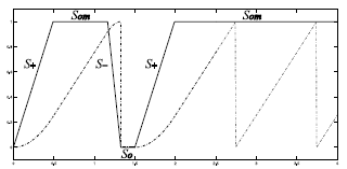
Figure 10 Green Wave Analysis. The dotted line refers to the normalized position and the solid dark line refers to the normalized speed. Source: The authors.
To calculate the fuel consumption of the vehicle when the green wave phenomenon occurs, it is necessary to consider that the driver stops once during the travel and achieves to pass all the traffic lights during the rest of the travel with the maximum permissible speed.
See in Figure 10 that the vehicle begins its path, but it is forced to stop in the following traffic light given that this is red, as indicated by the sine function, due to it is in its negative semi cycle, see also Figure 4. Then, the driver waits until the green light appears and thus, he/she can continue with his/her path through the road. For this case, it is necessary to calculate the fuel consumption used until beginning again its travel and add the consumption used in the rest of the sequence of traffic lights.
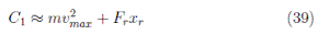
For the first part, the fuel consumption used is calculated between the first two traffic lights, which is similar to the calculated for the periodic orbit 1T , Equation (32).
Hence, the fuel consumption used between the first two traffic lights is determined by:
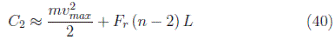
For the rest of the path, it is important to observe in Figure 10, that the automobile only shows two states S 0 and S +. Then, the fuel consumption C 2 is determined by the equation (40).
Thus, the total fuel consumption for the green wave can be expressed as:

Equations such as the shown (34), (35) and (38) can be formulated through modeling, simulation and dynamic analysis tools and use of maps; which will allow the scenario evaluation and analysis in future works facilitating the comprehension of emerging behaviors like those studied in this work.
6 Conclusions
A modeling diagram and a piecewise smooth system for a traffic system have been presented. To simulate this system, it is necessary to know the equations that describe its flow in each state and the conditions in the transition limits between the dynamic states. With this information and the bifurcation diagrams, it is possible to simulate a wide range of phenomena shown by this type of systems.
In the first stage, some numerical routines were illustrated in this document to simulate the hard-dynamic system. Periodic solutions, hard and soft bifurcations, fractals and chaos, just to mention some of the phenomena made evident, were obtained with these numerical simulations.
In the second stage, a stability analysis for two types of periodic orbits, which resulted being extremely stable was carried out. The fact that the periodic orbits 1T and 2T are extremely stable, they indicate that the system solutions do not differ under small modifications in the initial conditions. It is important to highlight the difference between a stable orbit and an extremely stable orbit with respect to the rate of convergence. The book Exploring Chaos: Theory and Experiment [15], establishes that a stable orbit has a linear rate of convergence and an extremely stable orbit has a quadratic rate of convergence.
Finally, an approximation of the fuel consumption was carried out through the use of a set of tools from the classical mechanics. This calculation was made for the following three types of solutions: periodic orbits 1T and 2T and the green wave. And with this, it was evidenced that the number of stops of a car through a road increases when the fuel consumption also increases. For this reason, configuring the traffic lights to obtain a green wave brings great benefits for the driver such as the reduction of travel time and fuel consumption, given that the number of stops is minimal.

